FrequencyDomain Adaptive Filters Wu Yihong EE 491 D

Frequency-Domain Adaptive Filters Wu, Yihong EE 491 D 5 -12 -2005

Overview n n n Advantages of FDAF Block-Adaptive Filters (BAF) Convergence Properties Choice of Block Size Methods Computational Complexity

Advantages of FDAF n n Providing a possible solution to the computational complexity problem Attaining a more uniform convergence rate by exploiting the orthogonality properties of DFT

Block-Adaptive Filters (BAF) n BAF Diagram n BLMS Equations n Convergence behavior

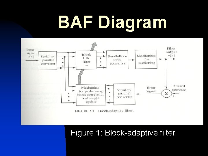
BAF Diagram Figure 1: Block-adaptive filter

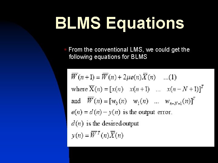
BLMS Equations § From the conventional LMS, we could get the following equations for BLMS

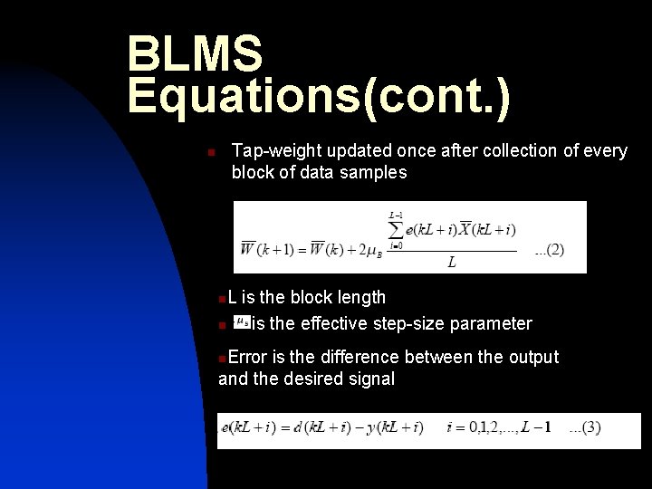
BLMS Equations(cont. ) Tap-weight updated once after collection of every block of data samples n L is the block length n is the effective step-size parameter n Error is the difference between the output and the desired signal n

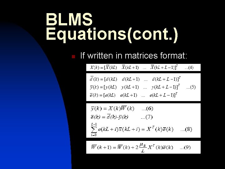
BLMS Equations(cont. ) n If written in matrices format:

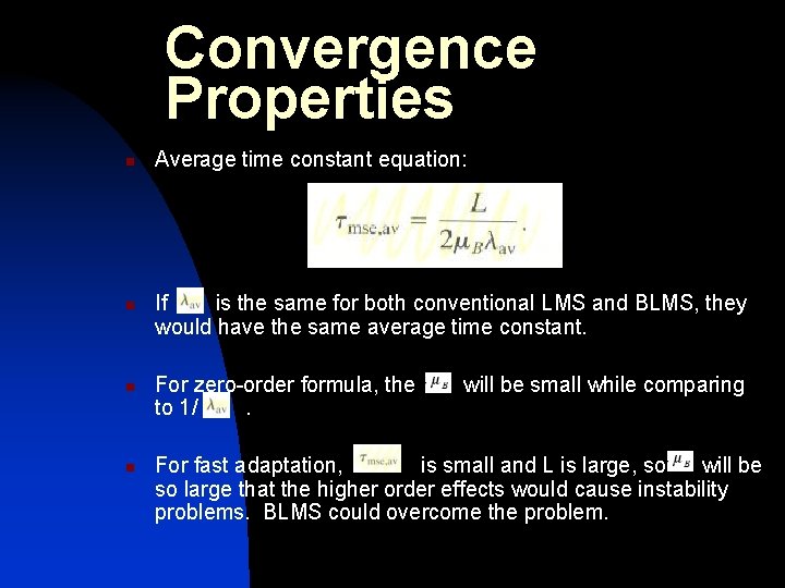
Convergence Properties n n Average time constant equation: If is the same for both conventional LMS and BLMS, they would have the same average time constant. For zero-order formula, the to 1/. will be small while comparing For fast adaptation, is small and L is large, so will be so large that the higher order effects would cause instability problems. BLMS could overcome the problem.

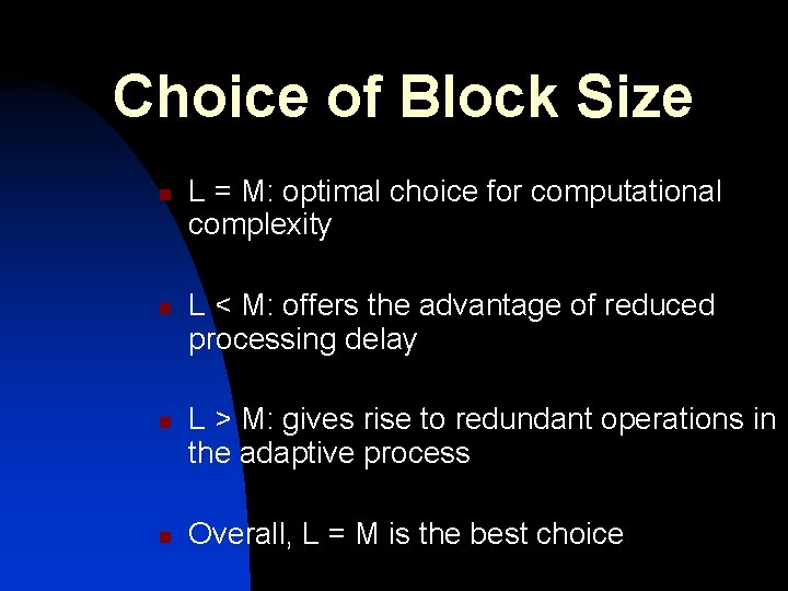
Choice of Block Size n n L = M: optimal choice for computational complexity L < M: offers the advantage of reduced processing delay L > M: gives rise to redundant operations in the adaptive process Overall, L = M is the best choice

Methods n Overlap-Save Sectioning n Overlap-Add Sectioning n Circular Convolution

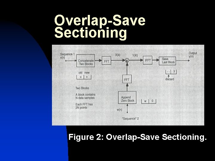
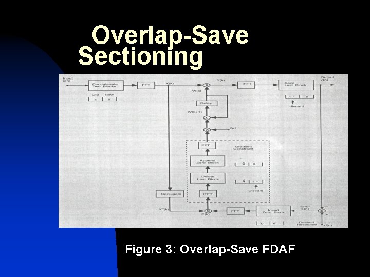
Overlap-Save Sectioning § Linear convolution between a finite-length sequence [w(n)]and an infinite-length sequence [x(n)]. § Zero-padding w(n) from N-point to 2 N-point § FFT both x(n) and w(n) to get Y(k) § First N point data would be ignored § Only looking for the last N point data

Overlap-Save Sectioning Figure 2: Overlap-Save Sectioning.

Overlap-Save Sectioning Figure 3: Overlap-Save FDAF

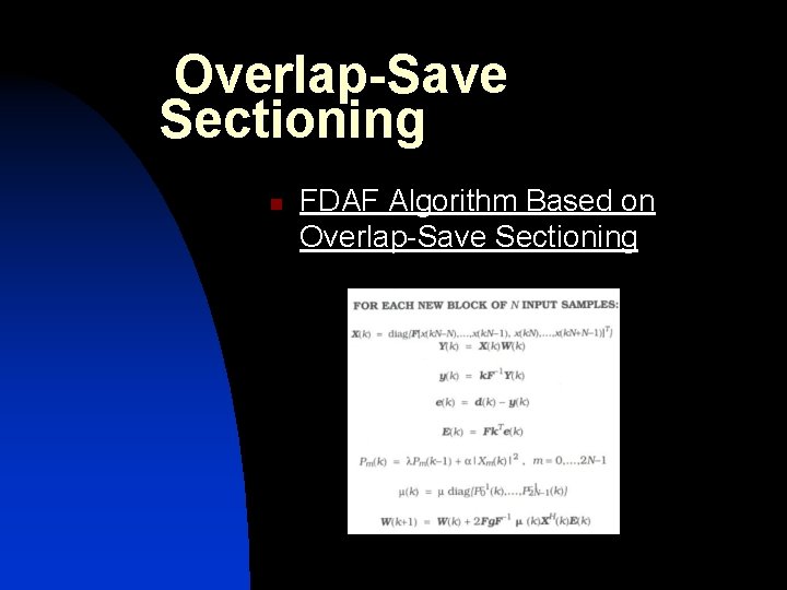
Overlap-Save Sectioning n FDAF Algorithm Based on Overlap-Save Sectioning

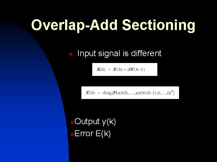
Overlap-Add Sectioning n Input signal is different Output y(k) n. Error E(k) n

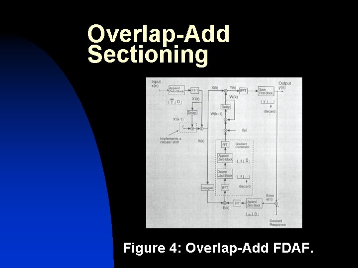
Overlap-Add Sectioning Figure 4: Overlap-Add FDAF.

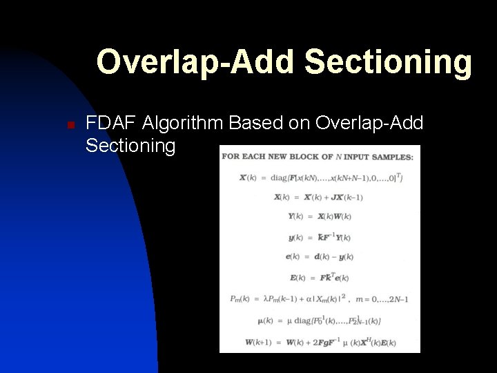
Overlap-Add Sectioning n FDAF Algorithm Based on Overlap-Add Sectioning

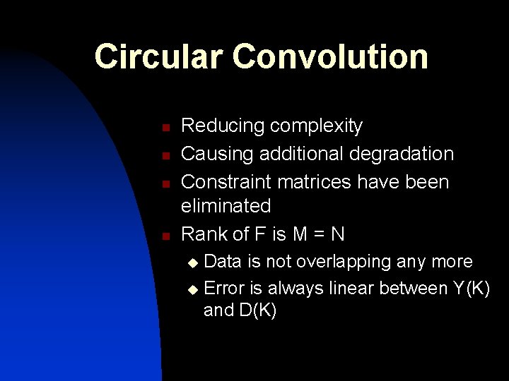
Circular Convolution n n Reducing complexity Causing additional degradation Constraint matrices have been eliminated Rank of F is M = N Data is not overlapping any more u Error is always linear between Y(K) and D(K) u

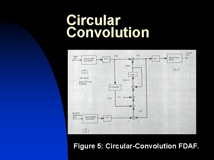
Circular Convolution Figure 5: Circular-Convolution FDAF.

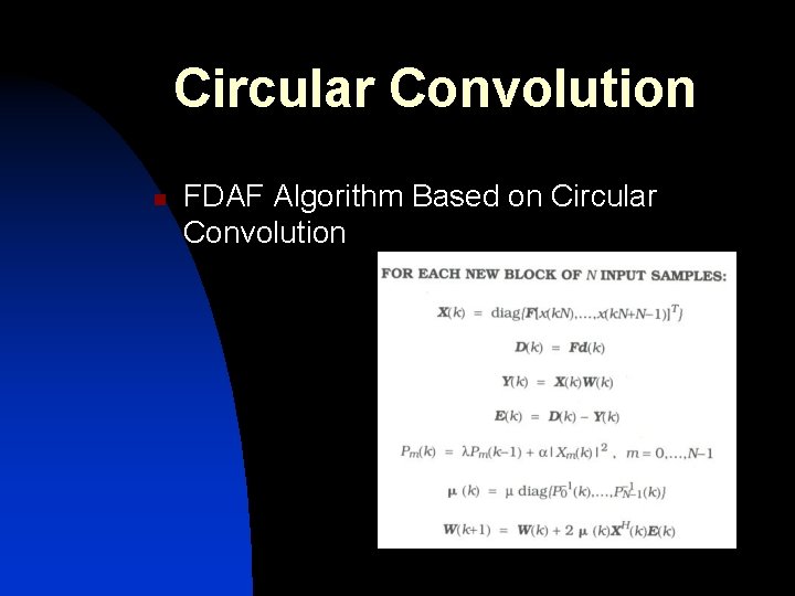
Circular Convolution n FDAF Algorithm Based on Circular Convolution

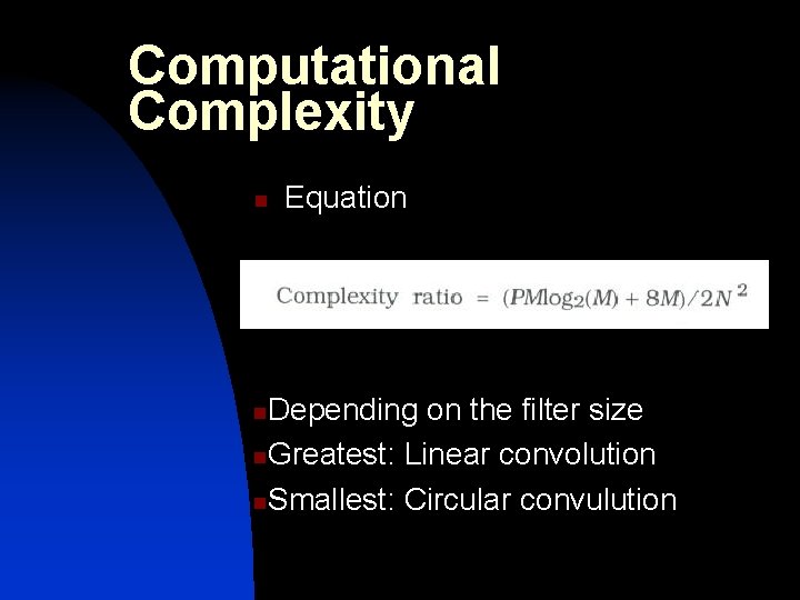
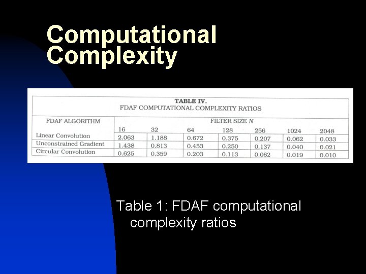
Computational Complexity n Equation Depending on the filter size n. Greatest: Linear convolution n. Smallest: Circular convulution n

Computational Complexity Table 1: FDAF computational complexity ratios

Conclusion n n Advantages of FDAF Computational Complexity Some methods Potential to be developed in the future

Thank you very much! Have a nice Summer!