Adaptive Filtering CHAPTER 4 Adaptive Tappeddelayline Filters Using

Adaptive Filtering CHAPTER 4 Adaptive Tapped-delay-line Filters Using the Least Squares

Adaptive Tapped-delay-line Filters Using the Least Squares In this presentation the method of least squares will be used to derive a recursive algorithm for automatically adjusting the coefficients of a tapped-delay-line filter, without invoking assumptions on the statistics of the input signals. This procedure, called the recursive least-squares (RLS) algorithm, is capable of realizing a rate of convergence that is much faster than the LMS algorithm, because the RLS algorithm utilizes all the information contained in the input data from the start of the adaptation up to the present.

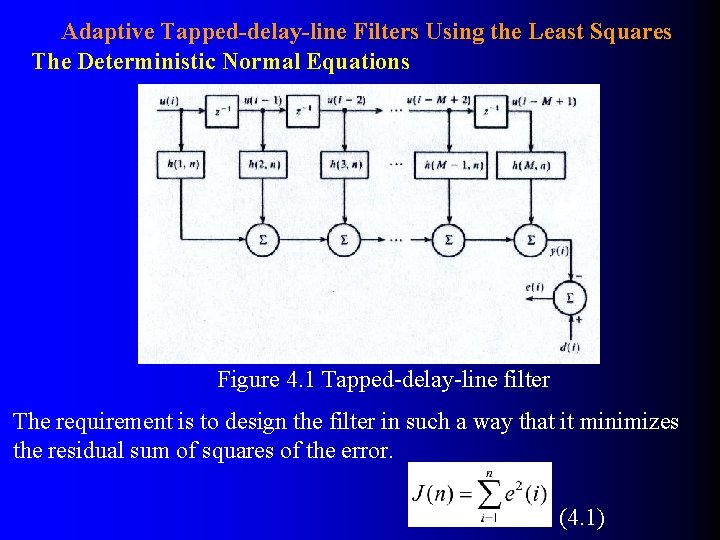
Adaptive Tapped-delay-line Filters Using the Least Squares The Deterministic Normal Equations Figure 4. 1 Tapped-delay-line filter The requirement is to design the filter in such a way that it minimizes the residual sum of squares of the error. (4. 1)

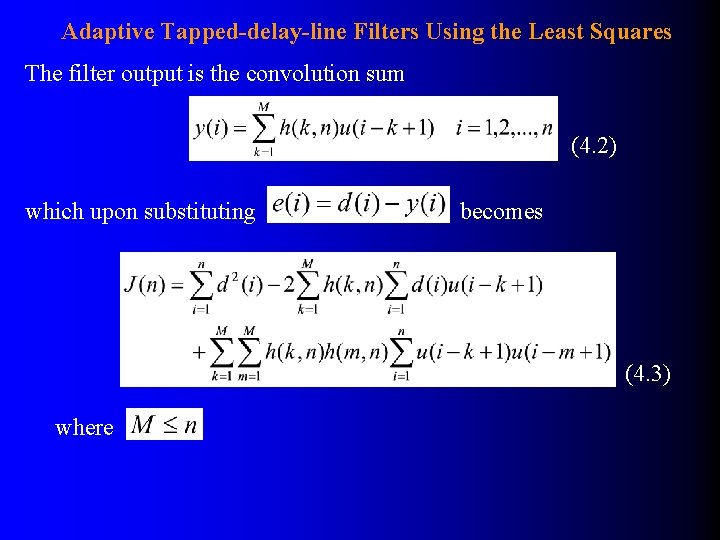
Adaptive Tapped-delay-line Filters Using the Least Squares The filter output is the convolution sum (4. 2) which upon substituting becomes (4. 3) where

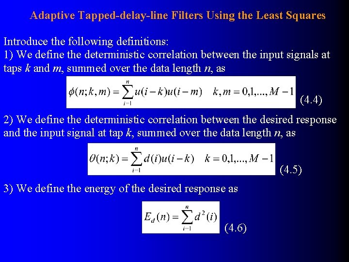
Adaptive Tapped-delay-line Filters Using the Least Squares Introduce the following definitions: 1) We define the deterministic correlation between the input signals at taps k and m, summed over the data length n, as (4. 4) 2) We define the deterministic correlation between the desired response and the input signal at tap k, summed over the data length n, as (4. 5) 3) We define the energy of the desired response as (4. 6)

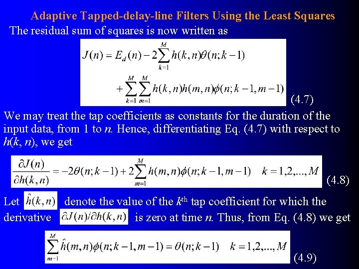
Adaptive Tapped-delay-line Filters Using the Least Squares The residual sum of squares is now written as (4. 7) We may treat the tap coefficients as constants for the duration of the input data, from 1 to n. Hence, differentiating Eq. (4. 7) with respect to h(k, n), we get (4. 8) Let derivative denote the value of the kth tap coefficient for which the is zero at time n. Thus, from Eq. (4. 8) we get (4. 9)

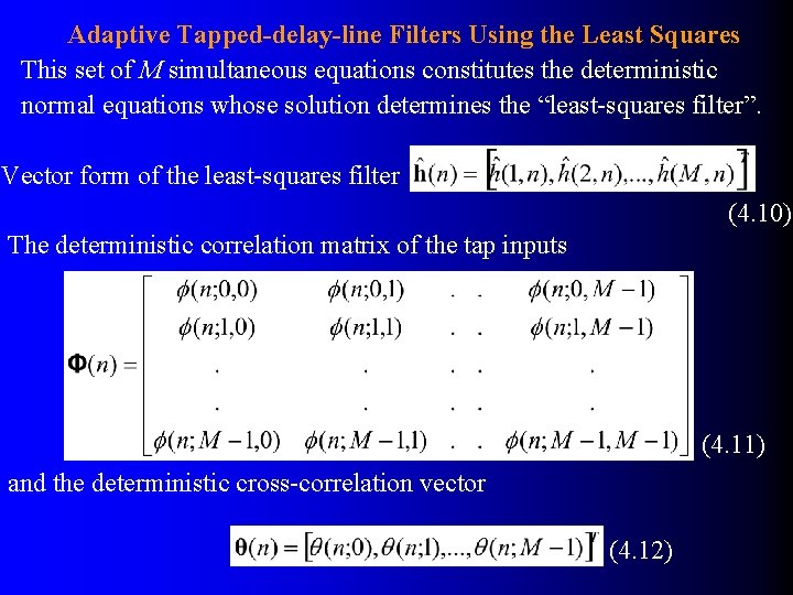
Adaptive Tapped-delay-line Filters Using the Least Squares This set of M simultaneous equations constitutes the deterministic normal equations whose solution determines the “least-squares filter”. Vector form of the least-squares filter (4. 10) The deterministic correlation matrix of the tap inputs (4. 11) and the deterministic cross-correlation vector (4. 12)

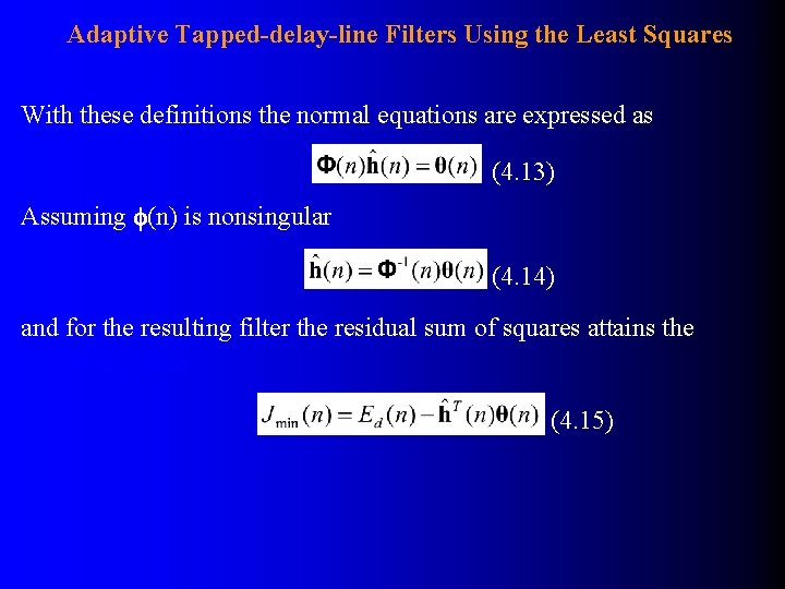
Adaptive Tapped-delay-line Filters Using the Least Squares With these definitions the normal equations are expressed as (4. 13) Assuming (n) is nonsingular (4. 14) and for the resulting filter the residual sum of squares attains the minimum value: (4. 15)

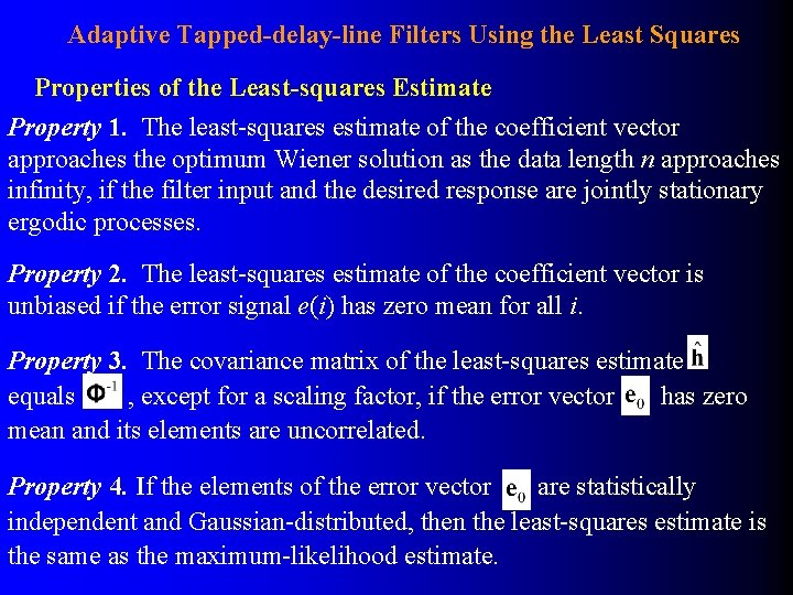
Adaptive Tapped-delay-line Filters Using the Least Squares Properties of the Least-squares Estimate Property 1. The least-squares estimate of the coefficient vector approaches the optimum Wiener solution as the data length n approaches infinity, if the filter input and the desired response are jointly stationary ergodic processes. Property 2. The least-squares estimate of the coefficient vector is unbiased if the error signal e(i) has zero mean for all i. Property 3. The covariance matrix of the least-squares estimate equals , except for a scaling factor, if the error vector has zero mean and its elements are uncorrelated. Property 4. If the elements of the error vector are statistically independent and Gaussian-distributed, then the least-squares estimate is the same as the maximum-likelihood estimate.

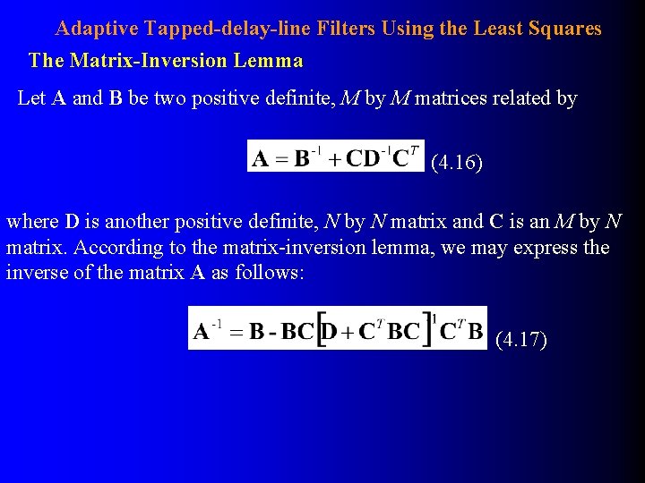
Adaptive Tapped-delay-line Filters Using the Least Squares The Matrix-Inversion Lemma Let A and B be two positive definite, M by M matrices related by (4. 16) where D is another positive definite, N by N matrix and C is an M by N matrix. According to the matrix-inversion lemma, we may express the inverse of the matrix A as follows: (4. 17)

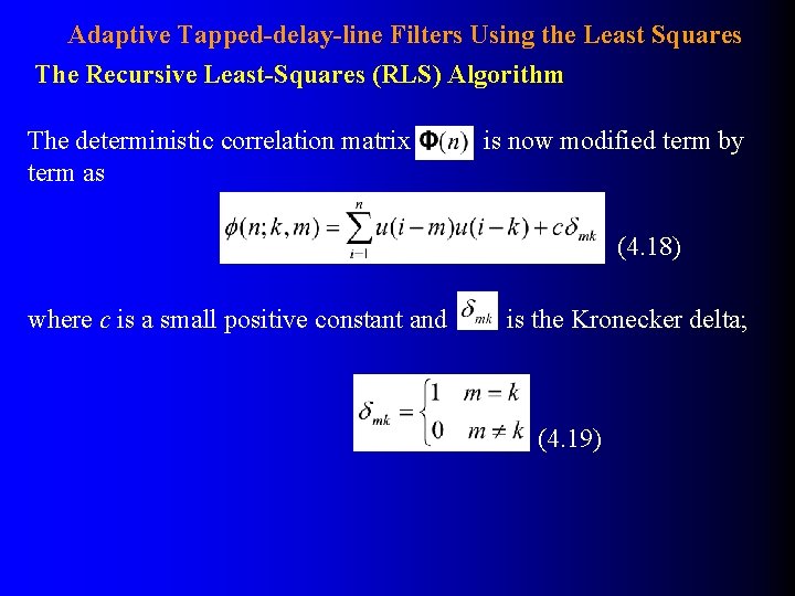
Adaptive Tapped-delay-line Filters Using the Least Squares The Recursive Least-Squares (RLS) Algorithm The deterministic correlation matrix term as is now modified term by (4. 18) where c is a small positive constant and is the Kronecker delta; (4. 19)

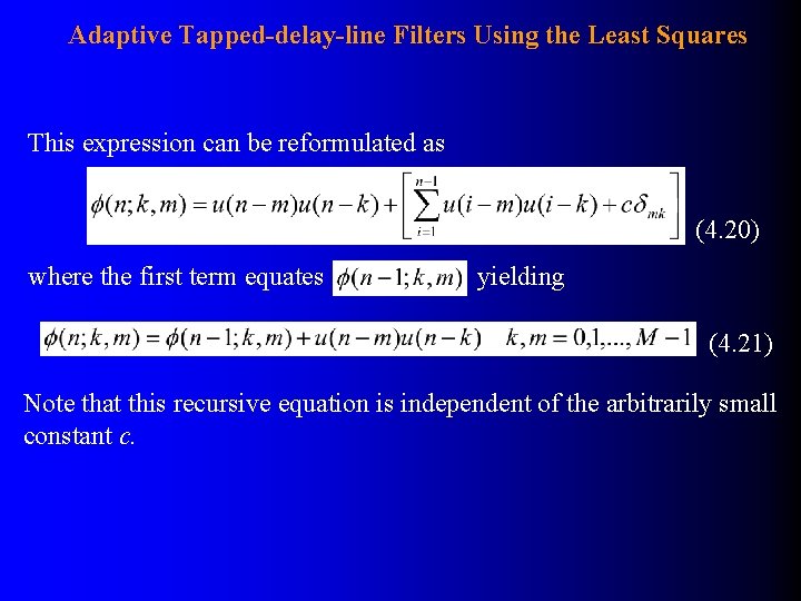
Adaptive Tapped-delay-line Filters Using the Least Squares This expression can be reformulated as (4. 20) where the first term equates yielding (4. 21) Note that this recursive equation is independent of the arbitrarily small constant c.

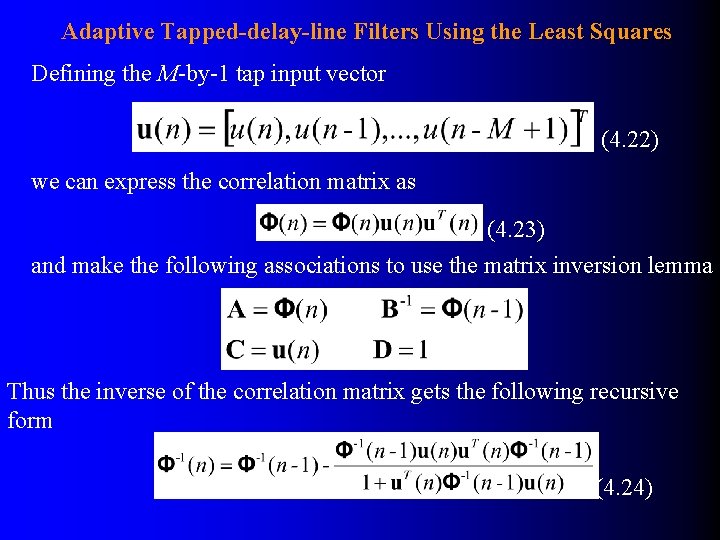
Adaptive Tapped-delay-line Filters Using the Least Squares Defining the M-by-1 tap input vector (4. 22) we can express the correlation matrix as (4. 23) and make the following associations to use the matrix inversion lemma Thus the inverse of the correlation matrix gets the following recursive form (4. 24)

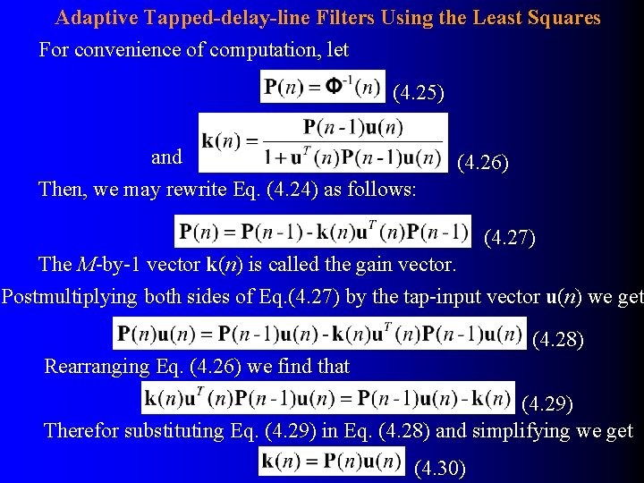
Adaptive Tapped-delay-line Filters Using the Least Squares For convenience of computation, let (4. 25) and Then, we may rewrite Eq. (4. 24) as follows: (4. 26) (4. 27) The M-by-1 vector k(n) is called the gain vector. Postmultiplying both sides of Eq. (4. 27) by the tap-input vector u(n) we get (4. 28) Rearranging Eq. (4. 26) we find that (4. 29) Therefor substituting Eq. (4. 29) in Eq. (4. 28) and simplifying we get (4. 30)

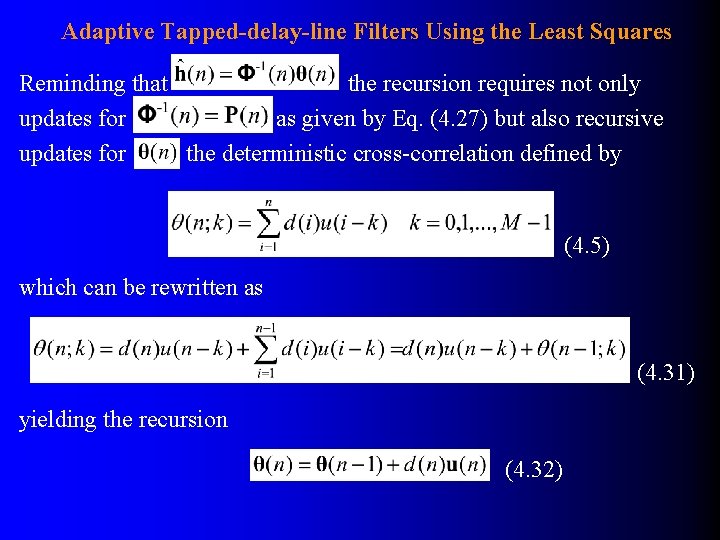
Adaptive Tapped-delay-line Filters Using the Least Squares Reminding that the recursion requires not only updates for as given by Eq. (4. 27) but also recursive updates for the deterministic cross-correlation defined by (4. 5) which can be rewritten as (4. 31) yielding the recursion (4. 32)

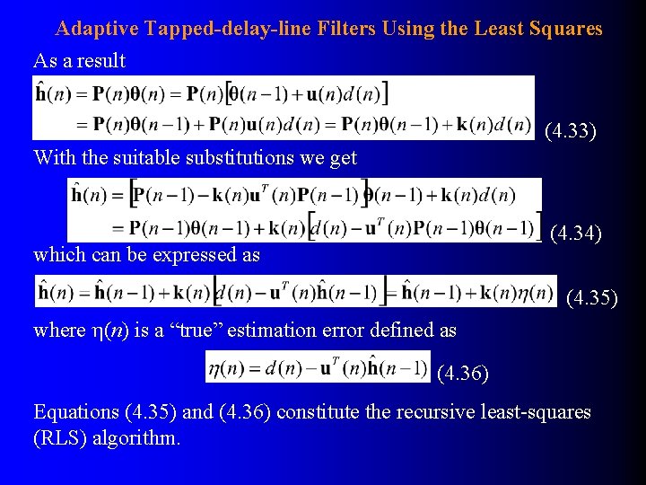
Adaptive Tapped-delay-line Filters Using the Least Squares As a result (4. 33) With the suitable substitutions we get (4. 34) which can be expressed as (4. 35) where (n) is a “true” estimation error defined as (4. 36) Equations (4. 35) and (4. 36) constitute the recursive least-squares (RLS) algorithm.

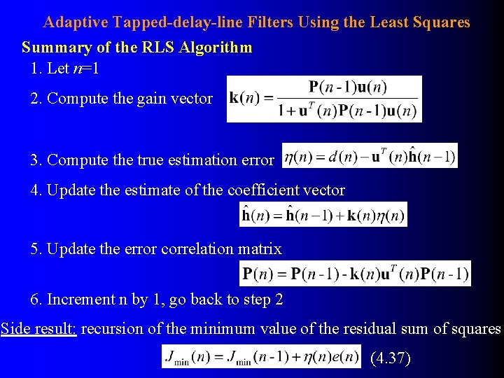
Adaptive Tapped-delay-line Filters Using the Least Squares Summary of the RLS Algorithm 1. Let n=1 2. Compute the gain vector 3. Compute the true estimation error 4. Update the estimate of the coefficient vector 5. Update the error correlation matrix 6. Increment n by 1, go back to step 2 Side result: recursion of the minimum value of the residual sum of squares (4. 37)

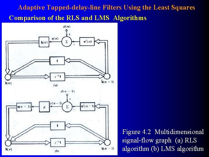
Adaptive Tapped-delay-line Filters Using the Least Squares Comparison of the RLS and LMS Algorithms Figure 4. 2 Multidimensional signal-flow graph (a) RLS algorithm (b) LMS algorithm

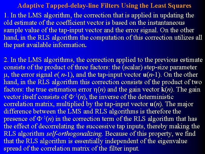
Adaptive Tapped-delay-line Filters Using the Least Squares 1. In the LMS algorithm, the correction that is applied in updating the old estimate of the coefficient vector is based on the instantaneous sample value of the tap-input vector and the error signal. On the other hand, in the RLS algorithm the computation of this correction utilizes all the past available information. 2. In the LMS algorithms, the correction applied to the previous estimate consists of the product of three factors: the (scalar) step-size parameter , the error signal e( n-1), and the tap-input vector u(n-1). On the other hand, in the RLS algorithm this correction consists of the product of two factors: the true estimation error (n) and the gain vector k(n). The gain vector itself consists of -1(n), the inverse of the deterministic correlation matrix, multiplied by the tap-input vector u(n). The major difference between the LMS and RLS algorithms is therefore the presence of -1(n) in the correction term of the RLS algorithm that has the effect of decorrelating the successive tap inputs, thereby making the RLS algorithm self-orthogonalizing. Because of this property, we find that the RLS algorithm is essentially independent of the eigenvalue spread of the correlation matrix of the filter input.

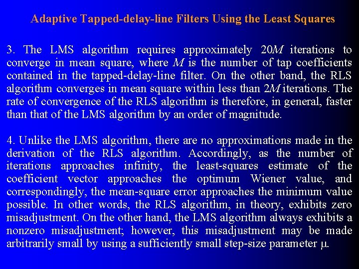
Adaptive Tapped-delay-line Filters Using the Least Squares 3. The LMS algorithm requires approximately 20 M iterations to converge in mean square, where M is the number of tap coefficients contained in the tapped-delay-line filter. On the other band, the RLS algorithm converges in mean square within less than 2 M iterations. The rate of convergence of the RLS algorithm is therefore, in general, faster than that of the LMS algorithm by an order of magnitude. 4. Unlike the LMS algorithm, there are no approximations made in the derivation of the RLS algorithm. Accordingly, as the number of iterations approaches infinity, the least-squares estimate of the coefficient vector approaches the optimum Wiener value, and correspondingly, the mean-square error approaches the minimum value possible. In other words, the RLS algorithm, in theory, exhibits zero misadjustment. On the other hand, the LMS algorithm always exhibits a nonzero misadjustment; however, this misadjustment may be made arbitrarily small by using a sufficiently small step-size parameter .

Adaptive Tapped-delay-line Filters Using the Least Squares 5. The superior performance of the RLS algorithm compared to the LMS algorithm, however, is attained at the expense of a large increase in computational complexity. The complexity of an adaptive algorithm for real-time operation is determined by two principal factors: (1) the number of multiplications (with divisions counted as multiplications) per iteration, and (2) the precision required to perform arithmetic operations. The RLS algorithm requires a total of 3 M(3 + M )/2 multiplications, which increases as the square of M, the number of filter coefficients. On the other hand, the LMS algorithm requires 2 M + 1 multiplications, increasing linearly with M. For example, for M = 31 the RLS algorithm requires 1581 multiplications, whereas the LMS algorithm requires only 63.