Energy Transformation 1 Caloria of heat energy necessary


 of precipitation • Arithmetic mean method – the rain gauge")


. High")

 • Meyboom method (Seasonal recession method): utilizes")
 • Rorabaugh method (Recession curve displacement method):")


. • dh/dl = Hydraulic gradient. • dh =")
 Turbulent flow")
. • K is also referred to")
. • K =")

2.")
![Permeameters • • Constant-head permeameter Qt = -[KAt(ha-hb)]/L. K = VL/Ath. V = volume](https://slidetodoc.com/presentation_image_h/d25fe85aac2b7850fa67b92f8e13e1f6/image-31.jpg "Permeameters • • Constant-head permeameter Qt = -[KAt(ha-hb)]/L. K = VL/Ath. V = volume")
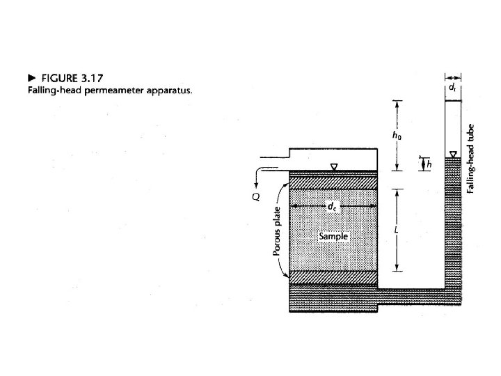
![Falling head permeameter • • K = [dt 2 L/dc 2 t]ln(h 0/h). K](https://slidetodoc.com/presentation_image_h/d25fe85aac2b7850fa67b92f8e13e1f6/image-33.jpg "Falling head permeameter • • K = [dt 2 L/dc 2 t]ln(h 0/h). K")


 Kv avg Kh avg Average")


- Slides: 51
Energy Transformation • 1 Caloria of heat = energy necessary to raise the temperature of one gram of pure water from 14. 5 – 15. 5 o. C • Latent Heat of vaporization Hv = 597. 3 – 0. 564 T (Cal. /g) • Latent Heat of condensation
Energy Transformation, Cont. • Latent heat of fusion – Hf – 1 g of ice at 0 o. C => ~80 cal of heat must be added to melt ice. Resulting water has same temperature. • Sublimation – Water passes directly from a solid state to a vapor state. Energy = Hf + Hv => 677 cal/g at 0 o. C. • Hv > 6 Hf > 5 x amt. to warm water from 0 o. C -> 100 o. C
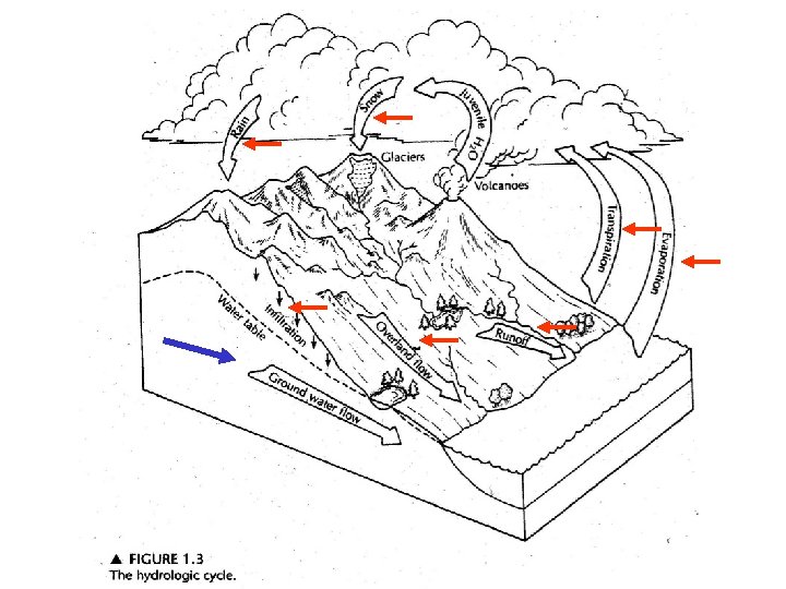
Hydrologic Equation • Inflow = outflow +/- Changes in storage • Equation is simple statement of mass conservation
Condensation • Condensation occurs when air mass can no longer hold all of its humidity. • Temperature drops => saturation humidity drops. • If absolute humidity remains constant => relative humidity rises. • Relative humidity reaches 100% => condensation => Dew point temperature.
Limited soil-moisture storage Cool, moist Warm, dry Cool, moist
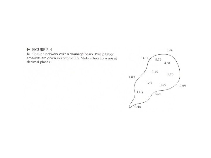
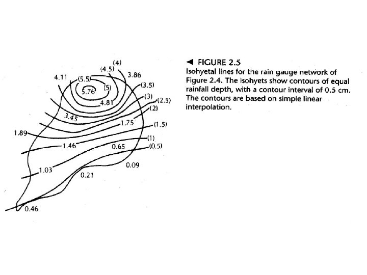
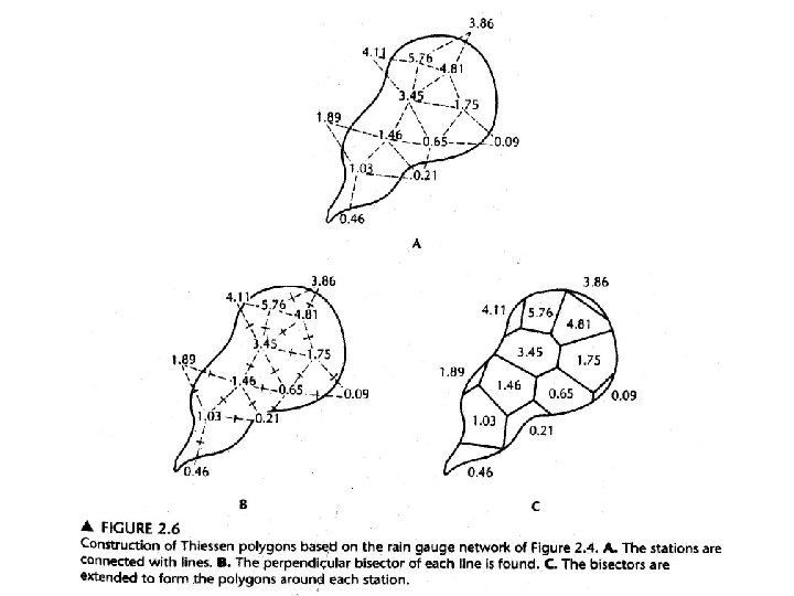
Effective uniform depth (EUD) of precipitation • Arithmetic mean method – the rain gauge network is of uniform density. • Isohyetal line method. • Thiessen method. - construct polygons - weighted by polygon areas
All infiltrate some water always on the surface All infiltrate Puddles and overland flow
Q 0
Increase of Recharge • • find t 1 tc = 0. 2144 t 1 find QA & QB Vtp = QBt 1/2. 3 – QAt 1/2. 3 • G = 2 Vtp
low overland return flows; high baseflow; strong water retaining (unconsolidated sand is thick). High overland return flows; low baseflow; little water retaining (soils are thin).
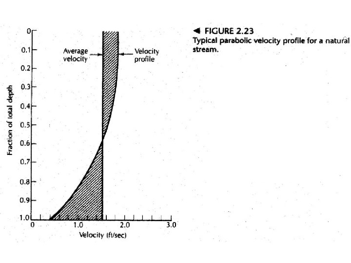
Manning equation • V = 1. 49 R 2/3 S 1/2 /n or R 2/3 S 1/2 /n • V – average velocity (L/T; ft/s or m/s). • R – hydraulic radius; or ratio of the crosssectional area of flow in square feet to the wetted perimeter (L; ft or m). • S – energy gradient or slope of the water surface. • n – the Manning roughness coefficient.
Determining ground water recharge from baseflow (1) • Meyboom method (Seasonal recession method): utilizes stream hydrographs from two or more consecutive years. • Assumptions: the catchment area has no dams or other method of streamflow regulation; snowmelt contributes little to the runoff.
Determining ground water recharge from baseflow (2) • Rorabaugh method (Recession curve displacement method): utilizes stream hydrograph during one season.
d 60 d 10
Sediment Classification • Sediments are classified on basis of size of individual grains • Grain size distribution curve • Uniformity coefficient Cu = d 60/d 10 • d 60 = grain size that is 60% finer by weight. • d 10 = grain size that is 10% finer by weight. • Cu = 4 => well sorted; Cu > 6 => poorly sorted.
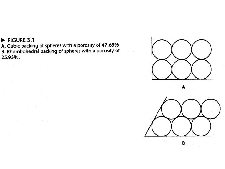
Specific Yield and Retention • Specific yield – Sy: ratio of volume of water that drains from a saturated rock owing to the attraction of gravity to the total volume of the rock. • Specific retention – Sr: ratio of the volume of water in a rock can retain against gravity drainage to the total volume of the rock. • n = S y + S r. • Sr increases with decreasing grain size.
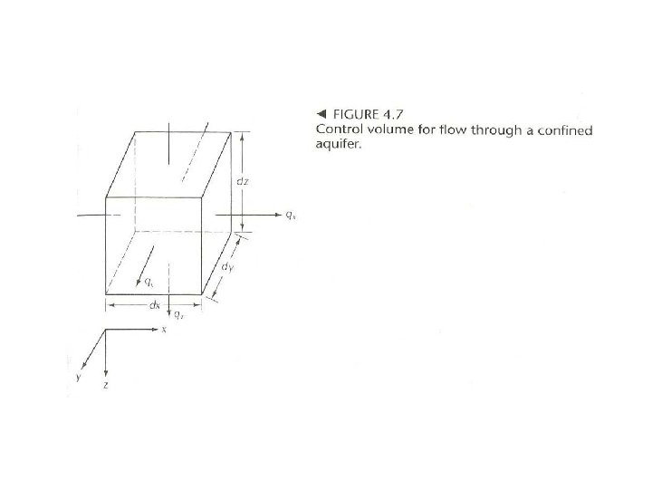
Darcy’s Law • Q = -KA(dh/dl). • dh/dl = Hydraulic gradient. • dh = change in head between two points separated by small distance dl.
Darcy’s Law: Yes Darcy’s Law: No Laminar flow (Small R < 10) Turbulent flow (Large R) Flow lines
Hydraulic conductivity • K = hydraulic conductivity (L/T). • K is also referred to as the coefficient of permeability. • K = -Q[A(dh/dl)] [ L 3/T/[L 2(L/L)] = L/T] • V = Q/A = -K(dh/dl) = specific discharge or Darcian velocity.
Intrinsic Permeability • Intrinsic permeability Ki = Cd 2 (L 2). • K = Ki (γ/μ) or K = Ki (ρg/ μ) • Petroleum industry 1 Darcy = unit of intrinsic permeability Ki • 1 darcy = 1 c. P x 1 cm 3/s / (1 atm/ 1 cm). c. P – centipoise - 0. 01 dyn s/cm 2 atm – atmospheric pressure – 1. 0132 x 1016 dyn/cm 2 • 1 darcy = 9. 87 x 10 -9 cm 2 ~ 10 -8 cm 2
Factors affecting permeability of sediments • Grain size increases permeability increases. • S. Dev. Of particle size increase poor sorting => permeability decrease. • Coarse samples show a greater decrease of permeability as S. Dev. Of particle size increases. • Unimodal samples (one dominant size) vs. bimodal samples.
Hazen method • Estimate hydraulic conductivity in sandy sediments. • K = C(d 10)2. • K = hydraulic conductivity. • d 10 = effective grain size (0. 1 – 3. 0 mm). • C = coefficient (see table on P 86).
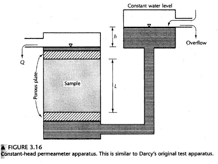
Permeameters • • Constant-head permeameter Qt = -[KAt(ha-hb)]/L. K = VL/Ath. V = volume of water discharging in time. L = length of the sample. A = cross-sectional area of sample. h = hydraulic head. K = hydraulic conductivity
Falling head permeameter • • K = [dt 2 L/dc 2 t]ln(h 0/h). K = Hydraulic conductivity. L = sample length. h 0 = initial head in the falling tube. h = final head in the falling tube. t = time that it takes for head to go from h 0 to h. dt = inside diameter of falling head tube. dc = inside diameter of sample chamber.
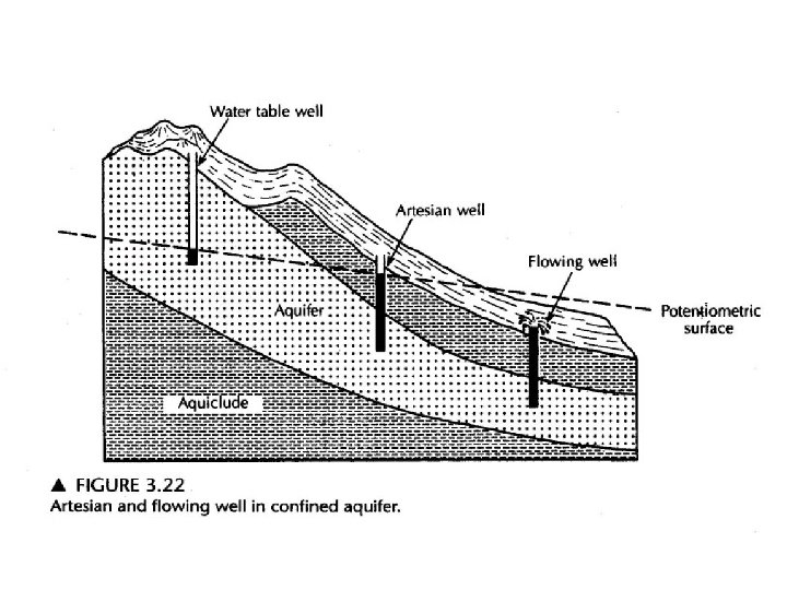
Aquifer • Aquifer – geologic unit that can store and transmit water at rates fast enough to supply amounts to wells. Usually, intrinsic permeability > 10 -2 Darcy. • Confining layer – unit with little or no permeability … < 10 -2 Darcy. aquifuge – absolutely impermeable unit. aquitard - a unit can store and transmit water slowly. Also called leaky confining layer. Raritan formation on Long Island. -- all these definitions are in a relative sense.
Transmissivity • The amount of water that can be transmitted horizontally through a unit width by the full saturated thickness of the aquifer under a hydraulic gradient of 1. • T = b. K • T = transmissivity. • b = saturated thickness. • K = hydraulic conductivity. • Multilayer => T 1 + T 2 + … + Tn
Specific Storage • Specific storage Ss = amount of water per unit volume stored or expelled owing to compressibility of mineral skeleton and pore water per unit change in head (1/L). • Ss = ρwg(α+nβ) • α = compressibiliy of aquifer skeleton. • n = porosity. • β = compressibility of water.
Storativity of confined Unit S = b Ss • Ss = specific storage. • b = aquifer thickness. • All water released in confined, saturated aquifer comes from compressibility of mineral skeleton and pore water.
Storativity in Unconfined Unit • Changes in saturation associated with changes in storage. • Storage or release depends on specific yield Sy and specific storage Ss. • S = Sy + b Ss
Volume of water drained from aquifer • • • Vw = SAdh Vw = volume of water drained. S = storativity (dimensionless). A = area overlying drained aquifer. dh = average decline in head.
Average horizontal conductivity: Kh avg = m=1, n (Khmbm/b) Kv avg Kh avg Average vertical conductivity: Kv avg = b / m=1, n (bm /Kvm)
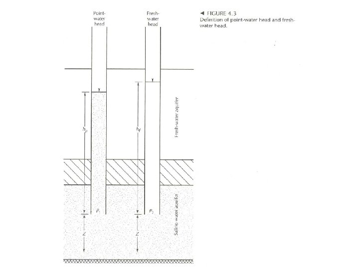
Hydraulic head, h • • Hydraulic head is energy per unit weight. h = v 2/2 g + z + P/gρ. [L]. Unit: (L; ft or m). v ~ 10 -6 m/s or 30 m/y for ground water flows. • v 2/2 g ~ 10 -12 m 2/s 2 / (2 x 9. 8 m/s 2) ~ 10 -13 m. • h = z + P/gρ. [L].
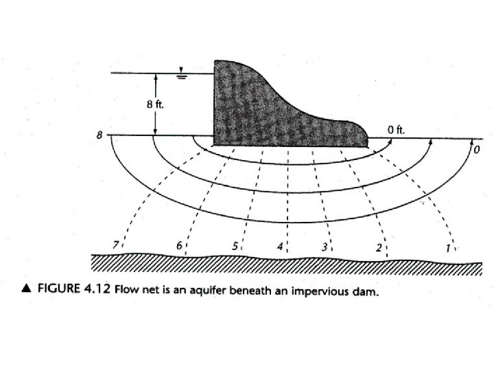
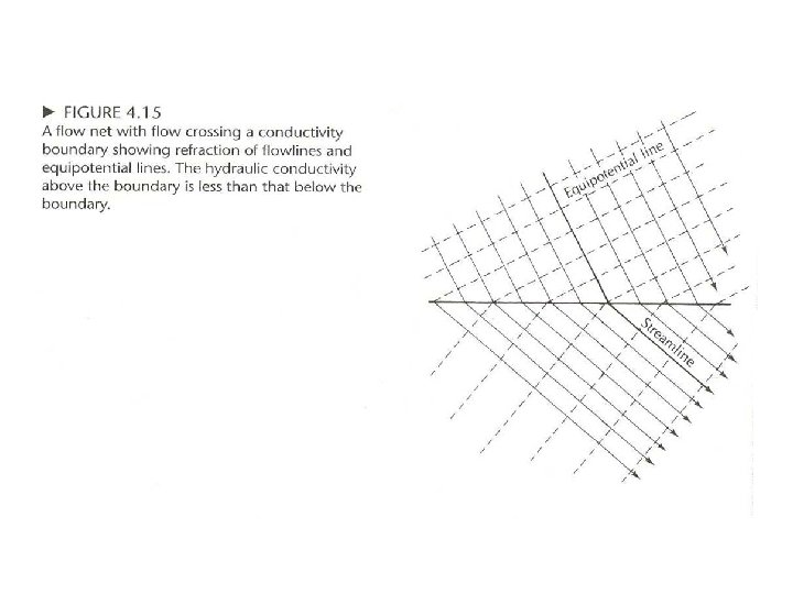
Flow lines and flow nets • A flow line is an imaginary line that traces the path that a particle of ground water would flow as it flows through an aquifer. • A flow net is a network of equipotential lines and associated flow lines.
Boundary conditions • No-flow boundary – flow line – parallel to the boundary. Equipotential line - intersect at right angle. • Constant-head boundary – flow line – intersect at right angle. Equipotential line - parallel to the boundary. • Water-table boundary – flow line – depends. Equipotential line - depends.
Estimate the quantity of water from flow net • q’ = Kph/f. • q’ – total volume discharge per unit width of aquifer (L 3/T; ft 3/d or m 3/d). • K – hydraulic conductivity (L/T; ft/d or m/d). • p – number of flowtubes bounded by adjacent pairs of flow lines. • h – total head loss over the length of flow lines (L; ft or m). • f - number of squares bounded by any two adjacent flow lines and covering the entire length of flow.