EECS 465 Digital Systems Lecture Notes 2 TwoLevel

EECS 465: Digital Systems Lecture Notes # 2 Two-Level Minimization Using Karnaugh Maps SHANTANU DUTT Department of Electrical & Computer Engineering University of Illinois, Chicago Phone: (312) 355 -1314: e-mail: dutt@ece. uic. edu URL: http: //www. ece. uic. edu/~dutt

Concepts in 2 -Level Minimization 2 • Defn: An implicant g of a function is a product term (e. g. , g=xyz) s. t. when g=1 f=1 • Defn: A minterm is an implicant whose product term representation consists of all n variables of an n-var. function (each in either compl. or uncompl. form) • Defn: Let g, and h be 2 implicants of a function f. g is said to cover h if h=1 g=1 (e. g. , g = xz, h = xyz) • Defn: Let G = {g 1, . . , gk} be a set of implicants of func f, and let h be another implicant of f. Then G covers h if h=1 g 1+. . + gk =1 (generalized covering).

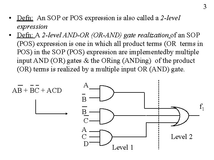
3 • Defn: An SOP or POS expression is also called a 2 -level expression • Defn: A 2 -level AND-OR (OR-AND) gate realization of an SOP (POS) expression is one in which all product terms (OR terms in POS) in the SOP (POS) expression are implementedby multiple input AND (OR) gates & the ORing (ANDing) of the product (OR) terms is realized by a multiple input OR (AND) gate. AB + BC + ACD A B B C A C D f 1 Level 2 Level 1

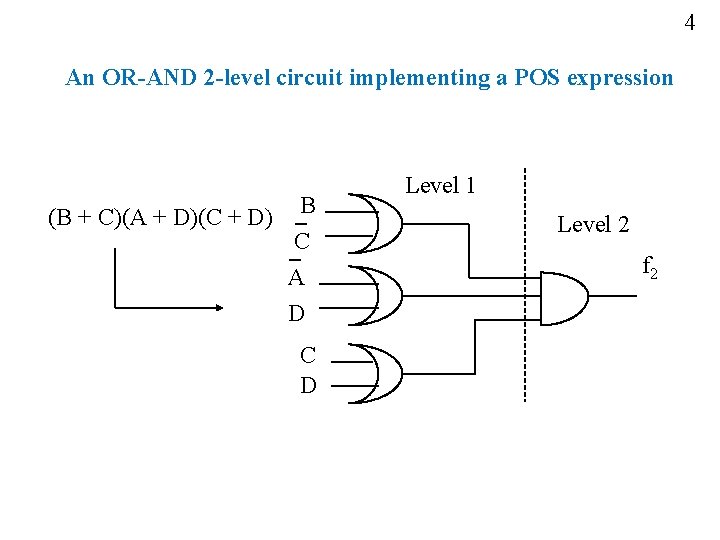
4 An OR-AND 2 -level circuit implementing a POS expression (B + C)(A + D)(C + D) B C A D C D Level 1 Level 2 f 2

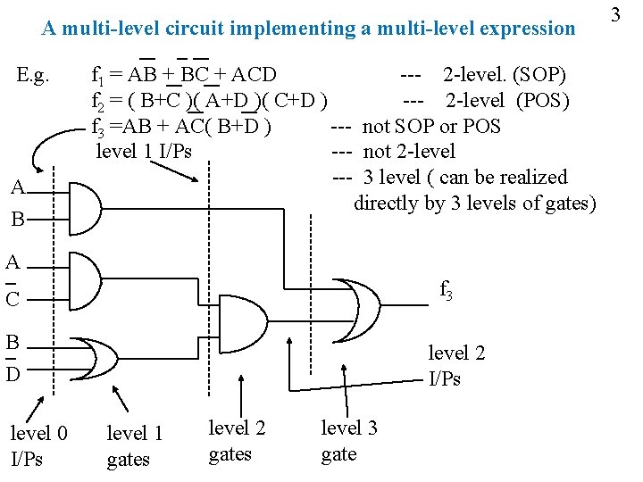
A multi-level circuit implementing a multi-level expression E. g. A B f 1 = AB + BC + ACD --- 2 -level. (SOP) f 2 = ( B+C )( A+D )( C+D ) --- 2 -level (POS) f 3 =AB + AC( B+D ) --- not SOP or POS level 1 I/Ps --- not 2 -level --- 3 level ( can be realized directly by 3 levels of gates) A f 3 C B D level 0 I/Ps level 2 I/Ps level 1 gates level 2 gates level 3 gate 3

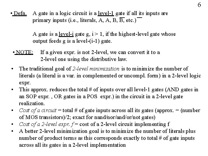
6 • Defn. A gate in a logic circuit is a level-1 gate if all its inputs are primary inputs (i. e. , literals, A, A, B, B, etc. ) A gate is a level-i gate g, i > 1, if the highest-level gate whose output feeds g is a level-(i-1) gate. • NOTE: If a given expr. is not 2 -level, we can convert it to a 2 -level one using the distributive law. • The traditional goal of 2 -level minimization is to minimize the number of literals (a literal is a var. in complemented or uncompl. form) in a 2 -level logic expr. • This approx. reduces the total # of inputs over all level-1 gates (AND gates in an SOP expr. , OR gates in a POS expr. ) in the circuit in a 2 -level gate realization. • Cost of a circuit = total # of gate inputs across all its gates (approx. = (number of MOS transistors)/2; exact for nand/nor/and/or/not gates) • Cost of a 2 -level expr. f = cost of a 2 -level circuit implementing f • A better 2 -level minimization goal is to minimize the number of literals plus number of product terms as this corresponds exactly to total # of gate inputs across all its gates in a 2 -level implementation

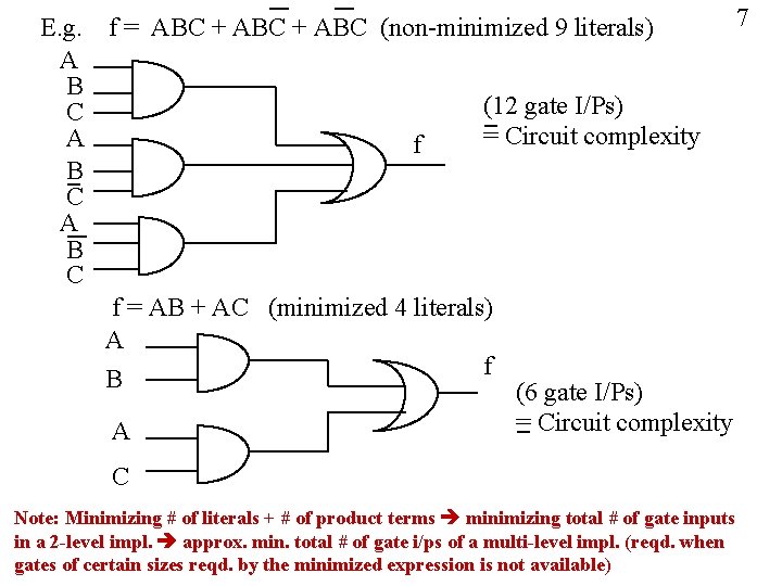
E. g. f = ABC + ABC (non-minimized 9 literals) A B (12 gate I/Ps) C = Circuit complexity A f B C A B C f = AB + AC (minimized 4 literals) A f B (6 gate I/Ps) A = Circuit complexity C Note: Minimizing # of literals + # of product terms minimizing total # of gate inputs in a 2 -level impl. approx. min. total # of gate i/ps of a multi-level impl. (reqd. when gates of certain sizes reqd. by the minimized expression is not available) 7

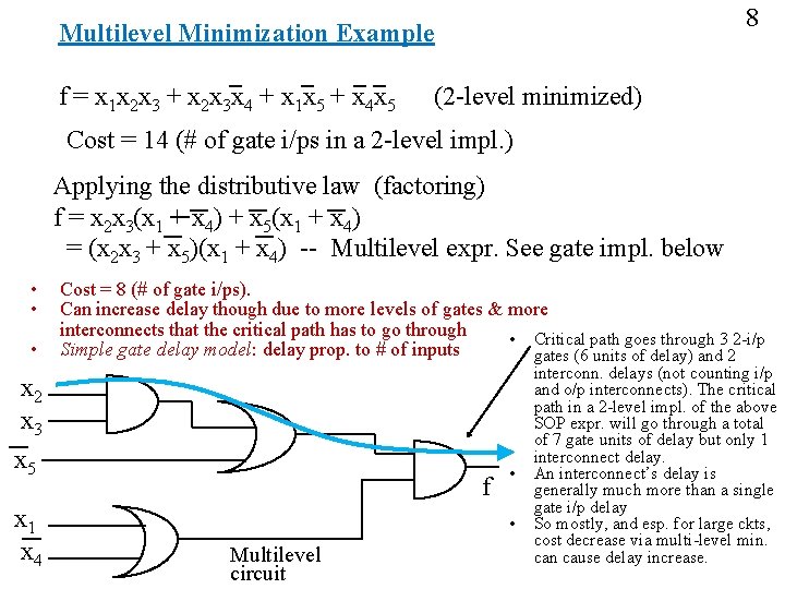
8 Multilevel Minimization Example f = x 1 x 2 x 3 + x 2 x 3 x 4 + x 1 x 5 + x 4 x 5 (2 -level minimized) Cost = 14 (# of gate i/ps in a 2 -level impl. ) Applying the distributive law (factoring) f = x 2 x 3(x 1 + x 4) + x 5(x 1 + x 4) = (x 2 x 3 + x 5)(x 1 + x 4) -- Multilevel expr. See gate impl. below • • • Cost = 8 (# of gate i/ps). Can increase delay though due to more levels of gates & more interconnects that the critical path has to go through • Critical path goes through 3 2 -i/p Simple gate delay model: delay prop. to # of inputs gates (6 units of delay) and 2 x 3 x 5 x 1 x 4 f • • Multilevel circuit interconn. delays (not counting i/p and o/p interconnects). The critical path in a 2 -level impl. of the above SOP expr. will go through a total of 7 gate units of delay but only 1 interconnect delay. An interconnect’s delay is generally much more than a single gate i/p delay So mostly, and esp. for large ckts, cost decrease via multi-level min. can cause delay increase.

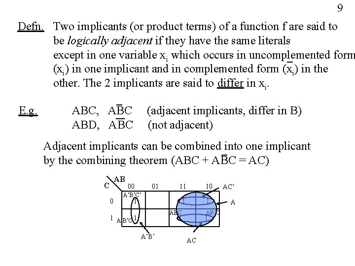
9 Defn. Two implicants (or product terms) of a function f are said to be logically adjacent if they have the same literals except in one variable xi which occurs in uncomplemented form (xi) in one implicant and in complemented form (xi) in the other. The 2 implicants are said to differ in xi. E. g. ABC, ABC ABD, ABC (adjacent implicants, differ in B) (not adjacent) Adjacent implicants can be combined into one implicant by the combining theorem (ABC + ABC = AC) AB C 0 00 01 11 10 1 1 A’B’C’ 1 ABC 1 A’B’C 1 A’B’ 1 AC AC’ A

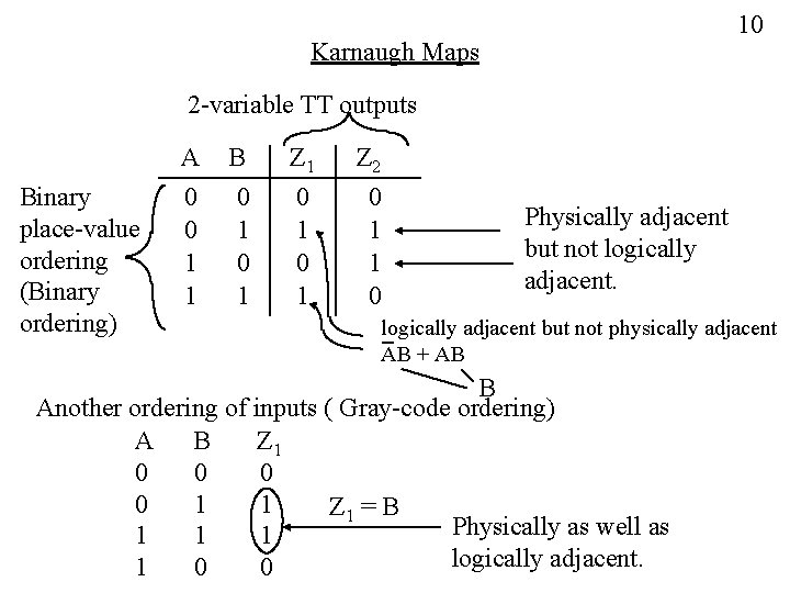
10 Karnaugh Maps 2 -variable TT outputs Binary place-value ordering (Binary ordering) A B Z 1 Z 2 0 0 1 1 0 1 0 1 0 1 1 0 Physically adjacent but not logically adjacent but not physically adjacent AB + AB B Another ordering of inputs ( Gray-code ordering) A B Z 1 0 0 1 1 Z 1 = B Physically as well as 1 1 1 logically adjacent. 1 0 0

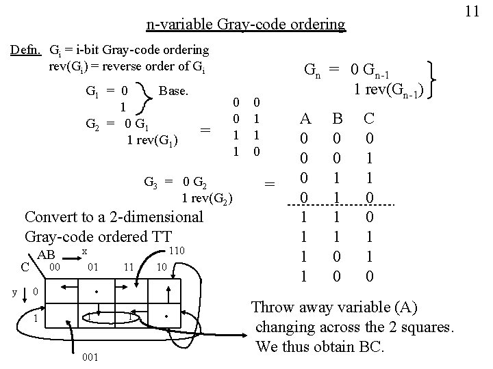
11 n-variable Gray-code ordering Defn. Gi = i-bit Gray-code ordering rev(Gi) = reverse order of Gi G 1 = 0 Base. 1 G 2 = 0 G 1 1 rev(G 1) = G 3 = 0 G 2 1 rev(G 2) Convert to a 2 -dimensional Gray-code ordered TT C y AB 00 x 110 01 10 1 • • 0 1 11 1 001 0 0 1 1 Gn = 0 Gn-1 1 rev(Gn-1) 0 1 1 0 = A 0 0 1 1 B 0 0 1 1 0 0 C 0 1 1 0 Throw away variable (A) changing across the 2 squares. We thus obtain BC.

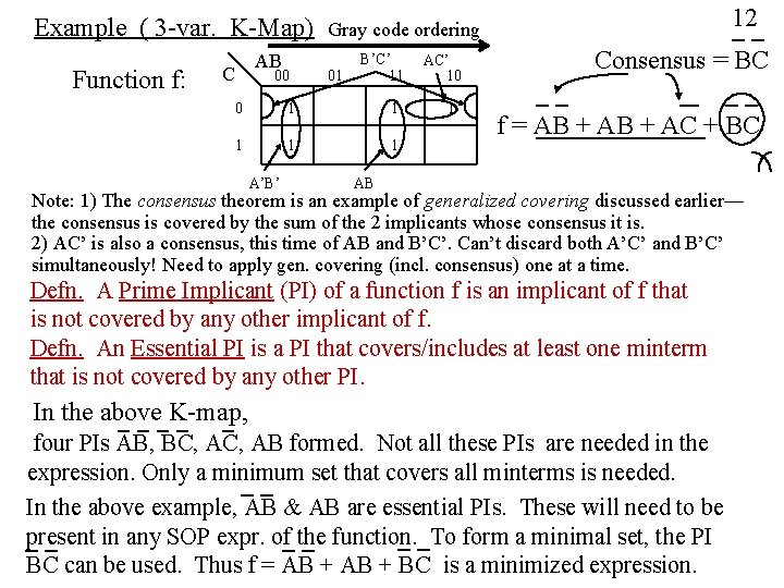
Example ( 3 -var. K-Map) Function f: AB C 00 01 B’C’ 11 0 1 1 1 A’B’ 12 Gray code ordering AC’ 10 1 Consensus = BC f = AB + AC + BC AB Note: 1) The consensus theorem is an example of generalized covering discussed earlier— the consensus is covered by the sum of the 2 implicants whose consensus it is. 2) AC’ is also a consensus, this time of AB and B’C’. Can’t discard both A’C’ and B’C’ simultaneously! Need to apply gen. covering (incl. consensus) one at a time. Defn. A Prime Implicant (PI) of a function f is an implicant of f that is not covered by any other implicant of f. Defn. An Essential PI is a PI that covers/includes at least one minterm that is not covered by any other PI. In the above K-map, four PIs AB, BC, AB formed. Not all these PIs are needed in the expression. Only a minimum set that covers all minterms is needed. In the above example, AB & AB are essential PIs. These will need to be present in any SOP expr. of the function. To form a minimal set, the PI BC can be used. Thus f = AB + BC is a minimized expression.

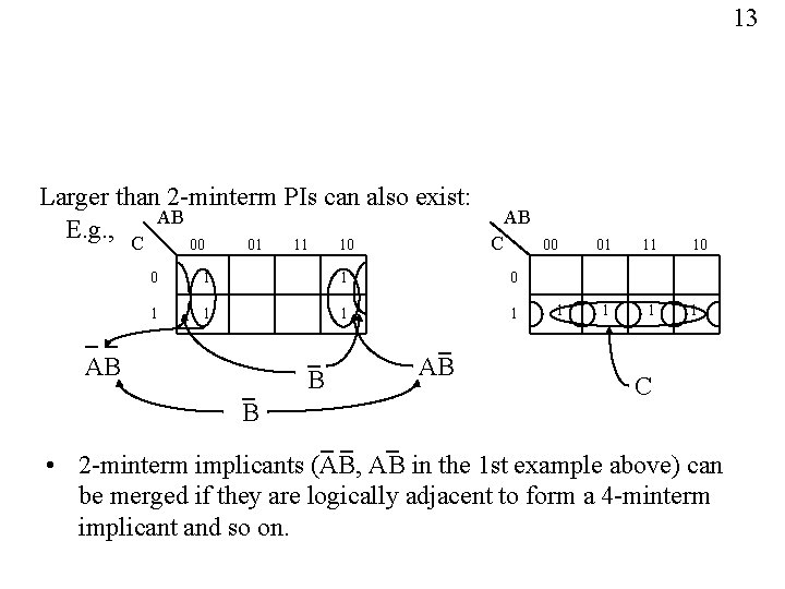
13 Larger than 2 -minterm PIs can also exist: AB E. g. , C 00 01 11 10 AB C 00 0 1 1 1 1 AB B B AB 1 01 11 1 1 10 1 C • 2 -minterm implicants (AB, AB in the 1 st example above) can be merged if they are logically adjacent to form a 4 -minterm implicant and so on.

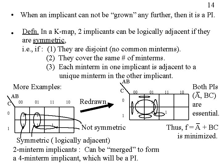
14 • When an implicant can not be “grown” any further, then it is a PI. Defn. In a K-map, 2 implicants can be logically adjacent if they are symmetric, i. e. , if : (1) They are disjoint (no common minterms). (2) They cover the same # of minterms. (3) Each minterm in one implicant is adjacent to a unique minterm in the other implicant. AB More Examples: Both PIs C 00 01 11 10 (A, BC) AB 0 01 11 10 1 1 Redrawn C 00 are 1 1 1 0 essential. 1 1 1 • 1 1 Not symmetric Symmetric ( logically adjacent) 2 -minterm implicants : Can be “merged” to form a 4 -minterm implicant, which will be a PI. Thus, f = A + BC is minimized.

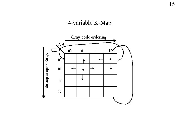
15 4 -variable K-Map: Gray code ordering AB CD 00 01 Gray code ordering 11 10 10 • 00 01 11 •

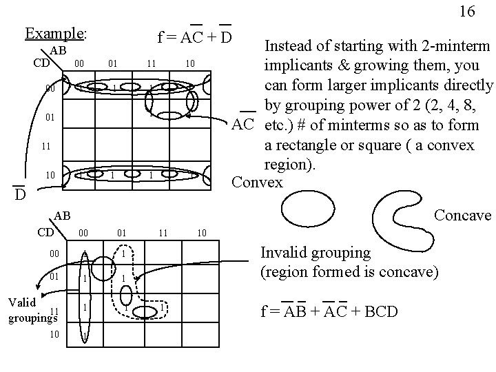
16 Example: f = AC + D AB CD 00 01 11 10 00 1 1 1 1 01 Instead of starting with 2 -minterm implicants & growing them, you can form larger implicants directly by grouping power of 2 (2, 4, 8, AC etc. ) # of minterms so as to form a rectangle or square ( a convex region). Convex 11 10 1 1 D Concave AB CD 00 01 00 1 1 01 1 1 Valid 11 groupings 1 1 10 1 11 10 Invalid grouping (region formed is concave) 1 f = AB + AC + BCD

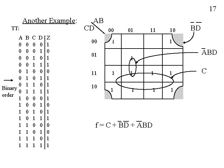
17 Another Example: TT: A 0 0 0 0 Binary 0 order 1 1 1 1 B 0 0 0 0 1 1 1 1 C 0 0 1 1 D 0 1 0 1 Z 1 0 1 1 1 1 0 0 1 1 AB CD 00 00 10 11 1 01 10 BD 1 ABD 1 1 1 1 1 f = C + BD + ABD C

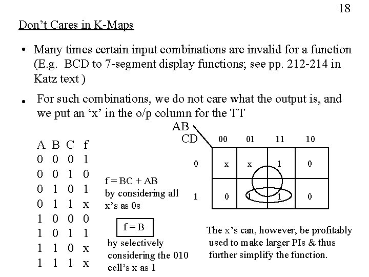
18 Don’t Cares in K-Maps • Many times certain input combinations are invalid for a function (E. g. BCD to 7 -segment display functions; see pp. 212 -214 in Katz text ) • For such combinations, we do not care what the output is, and we put an ‘x’ in the o/p column for the TT AB 00 01 11 10 CD A B C f 0 0 0 1 0 x x 1 0 0 0 1 0 f = BC + AB 0 1 by considering all 1 0 1 1 0 0 1 1 x x’s as 0 s 1 0 0 0 f=B The x’s can, however, be profitably 1 0 1 1 used to make larger PIs & thus 1 1 0 x by selectively further simplify the function. considering the 010 1 1 1 x cell’s x as 1

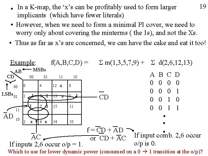
19 • In a K-map, the ‘x’s can be profitably used to form larger implicants (which have fewer literals) • However, when we need to form a minimal PI cover, we need to worry only about covering the minterms ( the 1 s), and not the Xs. • Thus as far as x’s are concerned, we can have the cake and eat it too! Example: CD 00 0 LSBs 01 1 11 10 S m(1, 3, 5, 7, 9) + S d(2, 6, 12, 13) MSBs AB 00 AD f(A, B, C, D) = 1 3 1 2 x 01 11 10 4 12 x 8 5 1 13 x 9 7 1 15 11 6 x 14 1 CD 10 AC If inputs 2, 6 occur o/p = 1. f = CD + AD or CD + AC A 0 0 B 0 0 C 0 0 1 1 D 0 1 • • • 2, 6 occur If input comb. o/p is 0. Which to use for lower dynamic power (consumed on a 0 1 transition at the o/p)?

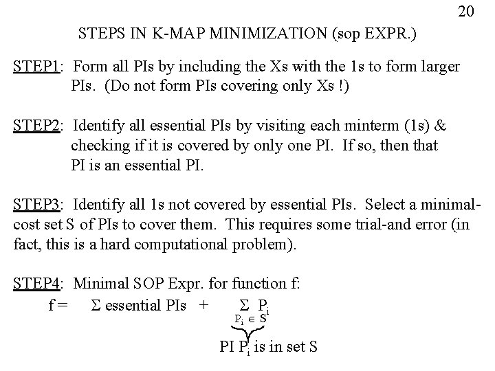
20 STEPS IN K-MAP MINIMIZATION (sop EXPR. ) STEP 1: Form all PIs by including the Xs with the 1 s to form larger PIs. (Do not form PIs covering only Xs !) STEP 2: Identify all essential PIs by visiting each minterm (1 s) & checking if it is covered by only one PI. If so, then that PI is an essential PI. STEP 3: Identify all 1 s not covered by essential PIs. Select a minimalcost set S of PIs to cover them. This requires some trial-and error (in fact, this is a hard computational problem). STEP 4: Minimal SOP Expr. for function f: f = S essential PIs + S Pi Pi Î S PI Pi is in set S

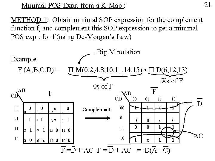
21 Minimal POS Expr. from a K-Map : METHOD 1: Obtain minimal SOP expression for the complement function f, and complement this SOP expression to get a minimal POS expr. for f (using De-Morgan’s Law) Big M notation Example: F (A, B, C, D) = AB CD 00 01 0 P M(0, 2, 4, 8, 10, 11, 14, 15) • P D(6, 12, 13) 0 s of F F 0 4 0 1 12 Xs of F CD x 13 x 8 00 01 11 10 00 1 1 x 1 1 01 0 0 x 1 0 1 1 x 1 1 0 Complement 1 1 5 11 3 1 7 1 15 0 11 10 2 0 6 x 14 0 10 9 F AB F =D + AC F = D + AC = D(A +C) D AC

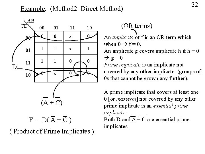
Example: (Method 2: Direct Method) AB CD 00 D 01 11 10 00 0 0 x 0 01 1 1 x 1 11 1 1 0 0 10 0 x 0 0 (A + C) F = D( A + C ) ( Product of Prime Implicates ) 22 (OR terms) An implicate of f is an OR term which when 0 f = 0. An implicate g covers implicate h if h = 0 g=0 Prime implicate is an implicate not covered by any other implicate. (groups of 0 s that cannot be grown any further). A prime implicate that covers at least one 0 [or maxterm] not covered by any other prime implicate is an essential prime implicate. Both D and A + C are essential prime implicates.

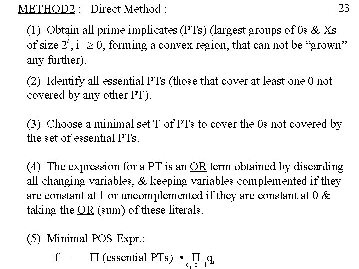
23 METHOD 2 : Direct Method : (1) Obtain all prime implicates (PTs) (largest groups of 0 s & Xs of size 2 , i ³ 0, forming a convex region, that can not be “grown” any further). (2) Identify all essential PTs (those that cover at least one 0 not covered by any other PT). (3) Choose a minimal set T of PTs to cover the 0 s not covered by the set of essential PTs. (4) The expression for a PT is an OR term obtained by discarding all changing variables, & keeping variables complemented if they are constant at 1 or uncomplemented if they are constant at 0 & taking the OR (sum) of these literals. (5) Minimal POS Expr. : f= P (essential PTs) • q P q Î T i i

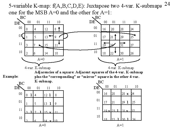
5 -variable K-map: f(A, B, C, D, E): Juxtapose two 4 -var. K-submaps 24 one for the MSB A=0 and the other for A=1: BC DE 00 01 11 10 DE BC 00 01 11 10 00 0 4 12 8 00 16 20 28 24 01 1 5 13 9 01 17 21 29 25 11 3 7 15 11 11 19 23 31 27 10 2 6 14 10 10 18 22 30 26 A=0 Example: BC DE 00 01 11 10 A=1 4 -var. K-submap Adjacencies of a square: Adjacent squares of the 4 -var. K-submap plus the “corresponding” or “mirror” square in the other 4 -var. K-submap. BC 00 01 11 10 0 1 4 12 1 8 1 13 1 9 5 3 1 7 1 15 x DE 00 01 11 11 10 2 6 14 x 10 A=0 00 01 11 10 16 20 28 x 24 17 21 29 1 25 31 x 27 22 1 30 1 26 19 x 23 1 18 A=1

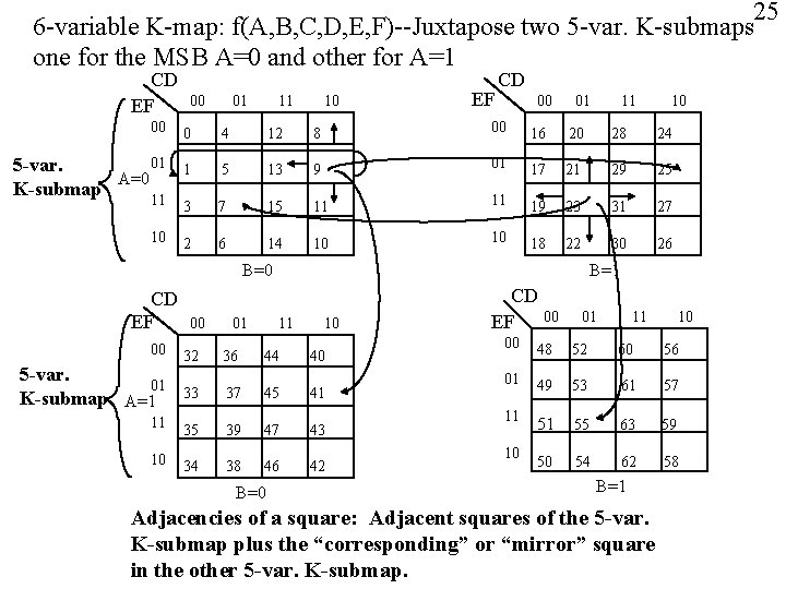
25 6 -variable K-map: f(A, B, C, D, E, F)--Juxtapose two 5 -var. K-submaps one for the MSB A=0 and other for A=1 CD EF 00 01 11 10 EF CD 00 01 11 10 00 0 4 12 8 00 16 20 28 24 01 5 -var. A=0 K-submap 1 5 13 9 01 17 21 29 25 11 3 7 15 11 11 19 23 31 27 10 2 6 14 10 10 18 22 30 26 B=0 CD EF 00 5 -var. 01 K-submap A=1 11 10 00 01 B=1 11 10 32 36 44 40 33 37 45 41 35 39 47 43 34 38 46 B=0 42 CD 00 EF 01 11 10 00 48 52 60 56 01 49 53 61 57 11 51 55 63 59 50 54 62 58 10 B=1 Adjacencies of a square: Adjacent squares of the 5 -var. K-submap plus the “corresponding” or “mirror” square in the other 5 -var. K-submap.

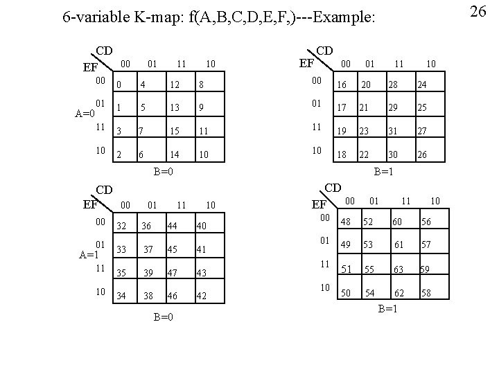
26 6 -variable K-map: f(A, B, C, D, E, F, )---Example: CD EF A=0 00 01 11 10 EF CD 00 01 11 10 00 0 4 12 8 00 16 20 28 24 01 1 5 13 9 01 17 21 29 25 11 3 7 15 11 11 19 23 31 27 10 2 6 14 10 10 18 22 30 26 B=0 CD EF 00 01 B=1 11 10 00 32 36 44 40 01 33 37 45 41 11 35 39 47 43 A=1 10 34 38 46 B=0 42 CD 00 EF 01 11 10 00 48 52 60 56 01 49 53 61 57 11 51 55 63 59 50 54 62 58 10 B=1

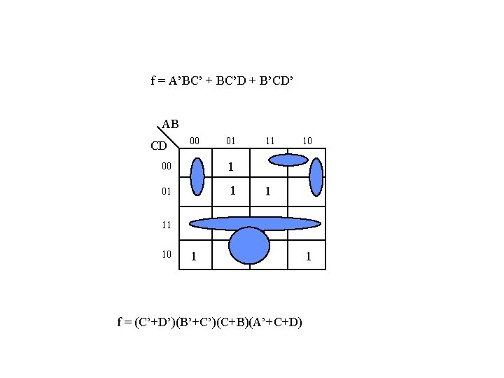
f = A’BC’ + BC’D + B’CD’ AB CD 00 01 00 1 01 1 11 10 1 f = (C’+D’)(B’+C’)(C+B)(A’+C+D) 1

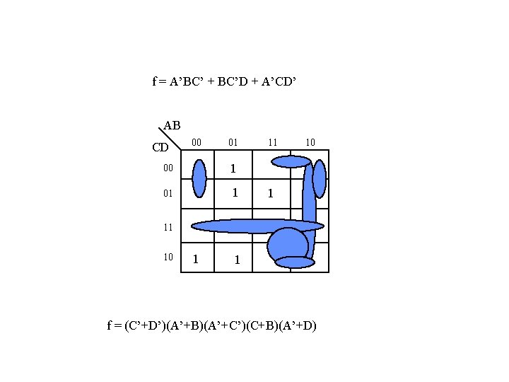
f = A’BC’ + BC’D + A’CD’ AB CD 00 01 00 1 01 1 11 10 1 1 f = (C’+D’)(A’+B)(A’+C’)(C+B)(A’+D)

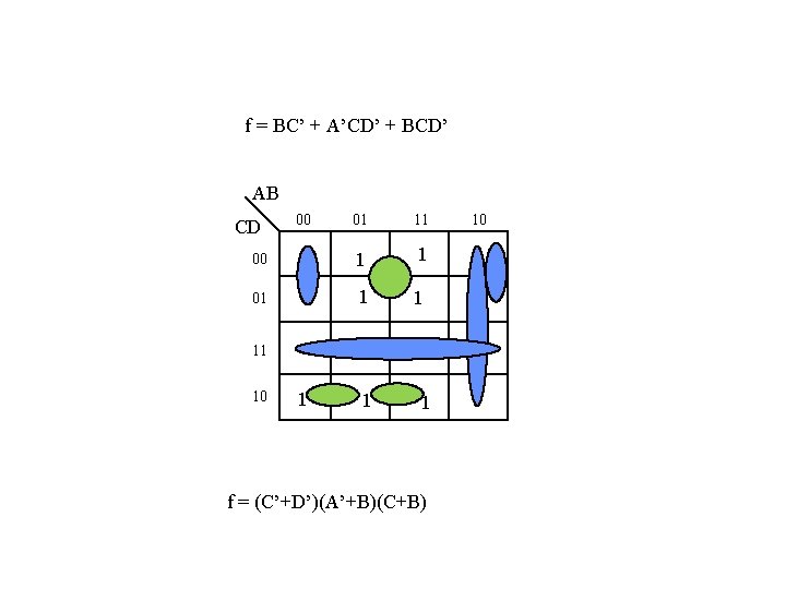
f = BC’ + A’CD’ + BCD’ AB 01 11 00 1 1 01 1 1 CD 00 11 10 1 1 1 f = (C’+D’)(A’+B)(C+B) 10