Economic History Master PPD APE Paris School of

Economic History (Master PPD & APE, Paris School of Economics) Thomas Piketty Academic year 2016 -2017 Lecture 3: The dynamics of capital accumulation: private vs public capital and the Great Transformation (check on line for updated versions)

Roadmap of lecture 3 • • • The measurement of national wealth The very long run: Britain and France, 1700 -2010 The rise and fall (and return? ) of foreign assets Private vs public capital: the Great transformation France, Britain, Germany, US: similarities & diffs Market vs book corporate values: capital & power Property regimes in history: from feudal to social Intellectual property and the public domain Natural capital and land prices From capital-income ratios to capital shares

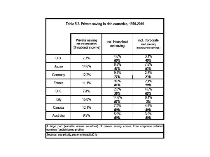
A quick summary of lecture 3 • Today we study the historical evolution of capital accumulation • Brief consensus during 1950 s-1980 s: steady-state balancedgrowth model, constant capital-output ratios β=K/Y and capital shares α=YK/Y • However if we take a longer run historical perspective, we find large variations in both β and α, due to many economic and political factors • Main lesson: asset prices and capital shares depend on the state of property relations, legal systems and bargaining power • « The Great Transformation » (Polanyi 1944): radical changes in attitudes toward private property during 1914 -1945 period: Great depression, bolshevik revolution, etc. • 1980 s-1990 s: fall of communism, financial deregulation, etc. : return to 19 c private-property-sacralization regime? Yes to some extent, but not so simple

The measurement of national wealth • Long tradition of national wealth estimates in Britain and France in the 18 th-19 th centuries: Britain: Petty, King, Giffen, etc. ; France: Vauban, Lavoisier, Colson, etc. (see Giffen 1889) • National balance sheets = estimates of all assets and liabilities held by residents of a country (and by the government) ( « Bilans patrimoniaux par pays » ) (see Goldsmith 1985, 1991) • Historical estimates are not sufficientely precise to study shortrun fluctuations; but they are fine to study broad orders of magnitudes and long-run evolutions • Recent estimates can be used to study short-run fluctuations: return to national balance sheets since 2008 financial crisis • See official UN methodological guides for measurement of national income and wealth: System of National Accounts 2008 • See Piketty-Zucman « Capital is Back – Wealth-Income Ratios in Rich Countries 1700 -2010 » , QJE 2014, Data Appendix, Database, for detailed bibliography and methodological issues

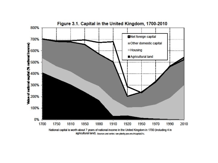
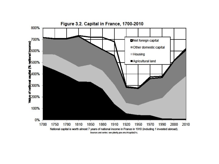
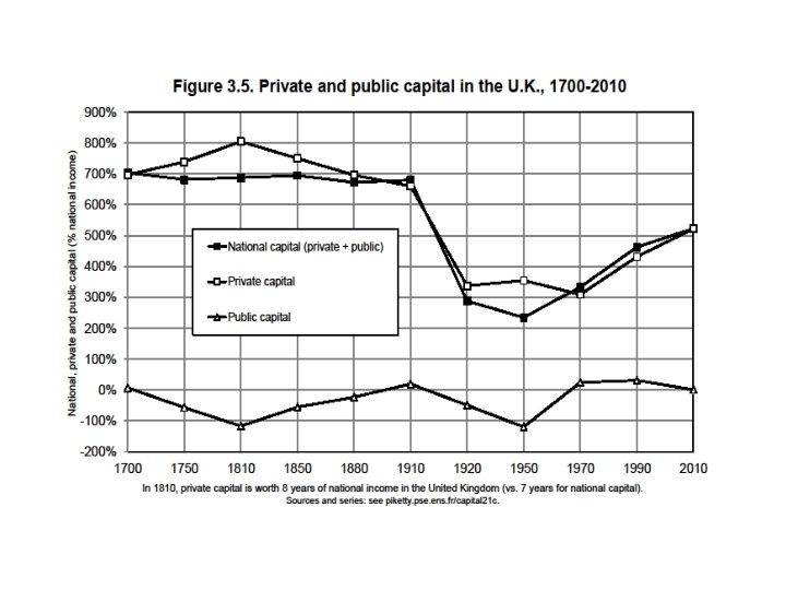
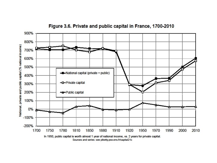
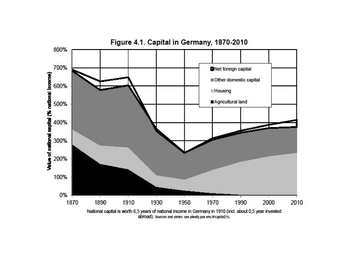
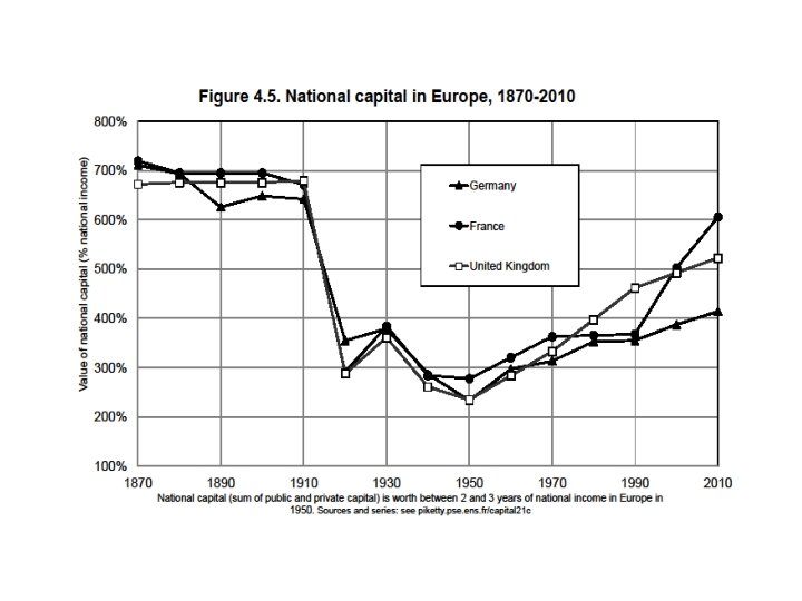
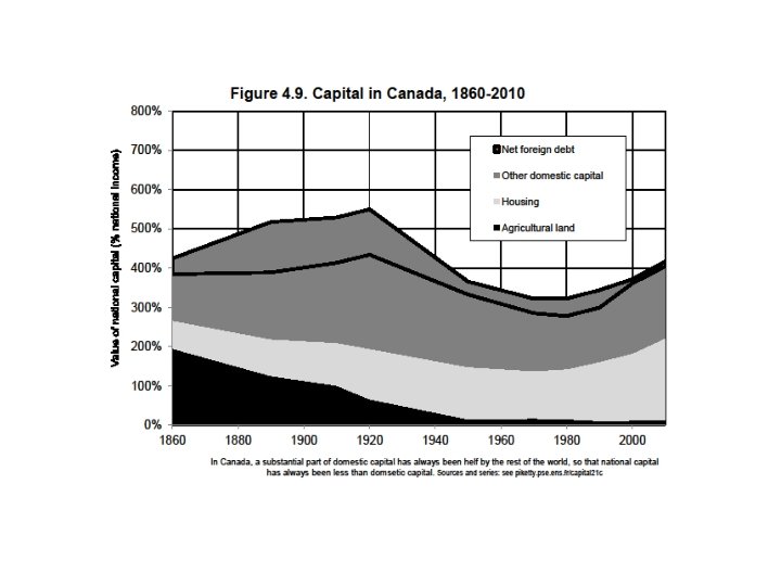
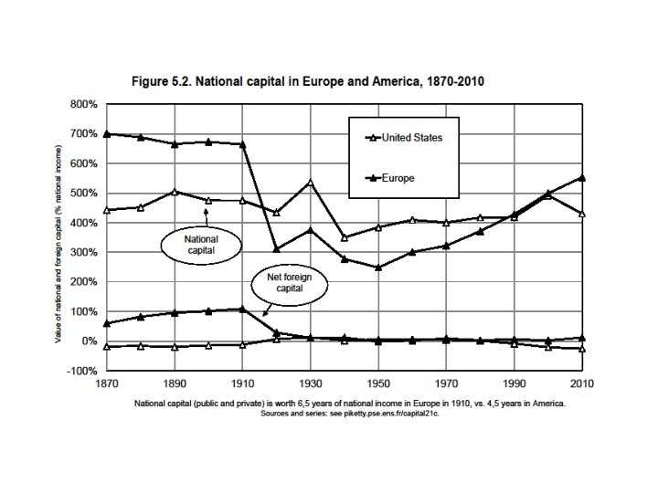
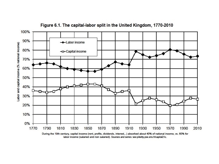
The very long-run: Britain and France 1700 -2010 • Longest series: Britain and France national wealth/national income ratio βn=Wn/Y over 1700 -2010 • National wealth Wn = Private wealth W + Public (or government) wealth Wg • Wn = Domestic capital K + Net foreign assets NFA • Domestic capital K = agricultural land + residential housing + other domestic k (=offices, structures, machines, patents, etc. used by firms and administrations) • Two major facts: (1) huge U-shaped curve: βn≈700% over 1700 -1910, down to 200 -300% around 1950, up to 500600% in 2000 -2010 (2) Radical change in the nature of wealth (agricultural land has been gradually replaced by housing, business and financial capital), but total value of wealth did not change that much in the very long run

The rise and fall of foreign assets • NFA close to 0 in 1700 -1800 and 1950 -2010, but very large in 1870 -1910 = the height of the « first globalization » and of colonial empires • In 1910, NFA≈200% of Y in UK, ≈100% in France • These enormous net foreign assets disappeared between 1910 and 1950 and never reappeared (but large cross-border gross positions developed since 1970 s-80 s: « second globalization » ) • 2010: Y ≈ 30 000€, Wn ≈ 180 000€ (βn≈ 6), including 90 000€ in housing and 90 000€ in other domestic k (financial assets invested in firms and govt) • 1700: assume Y ≈ 30 000€, then Wn ≈ 210 000€ (βn≈ 7), including 150 000€ in agricultural land 60 000€ in housing and other domestic capital • 1910 (UK): assume Y ≈ 30 000€, then Wn ≈ 210 000€ (βn≈ 7), including 60 000€ in housing, 90 000€ in other domestic capital and 60 000€ in net foreign assets

• With NFA as large as 100 -200% Y, the net foreign capital income is very large: around 1900 -1910, as large as 5% Y in France and 10% Y in Britain (average rate of return r=5%) • In effect, both countries were able to have permanent trade deficits (about 2% Y in 1870 -1910) and still to have a current account surplus and to accumulate more foreign reserves; i. e. they were consuming more than they what were producing, and at the same time they were getting richer • Today’s NFA for Japan-Germany-China (50 -100% Y) are smaller than Britain-France 1910, but are rising fast (more on this below, see figures 1970 -2010) • Three conclusions: (1) it’s nice to be a owner; (2) there’s no point accumulating trade surpluses for ever; (3) capital & property relations are also about power

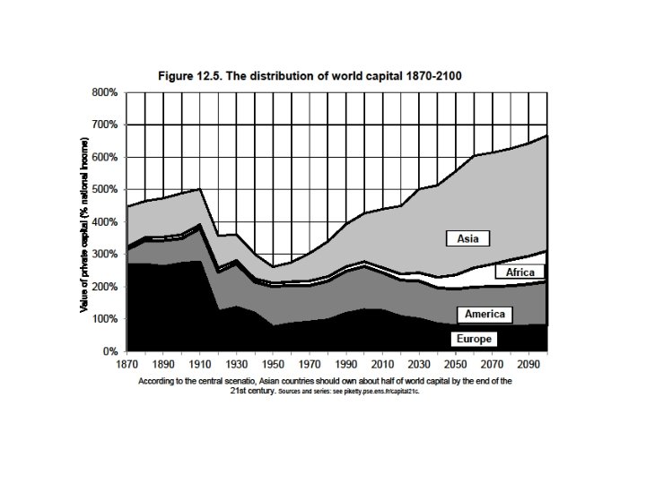
The return of foreign assets ? • How big were foreign assets in 1913, and how do they compare to today? Some simple computations (see Capital…, chap. 1) • In 1913, rich countries (Europe-America) made about 70% of world GDP, but about 75% of world income; poor countries (Asia-Africa) made about 30% of world GDP, but 25% of world income; this would mean that about 15% of poor countries’ output went abroad, i. e. 50% of their k income (assuming k share ≈ 30% GDP ): rich countries owned about 50% of poor countries capital in 1913 • Today: in Africa, GNI/GDP ratios have fluctuated around 95% over 1970 -2010 period according to WB series; this would mean that rich countries own about 20% of Africa’s capital today (and maybe 30 -50% if we exclude housing & land) (aid flows here) • Very approximate, ignores tax havens, includes only official flows

Gross vs net foreign assets: financial globalization in action • Net foreign asset positions are smaller today than what they were in 1900 -1910 • But they are rising fast in Germany, Japan and oil countries • And gross foreign assets and liabilities are a lot larger than they have ever been, especially in small countries • This potentially creates substantial financial fragility (especially if link between private risk and sovereign risk) • This destabilizing force is probably even more important than the rise of inequality: see lecture 6 • The structural evolution of NFA is determined not only by volume effects (trade & income balance) but also by price effects: capital gains and losses on foreign assets & liabilities (see PZ QJE 2014 and Gourinchas-Rey 2007)

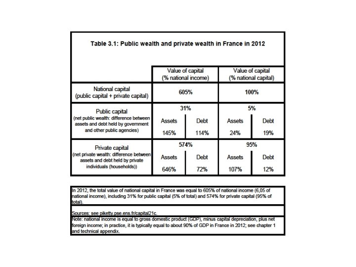
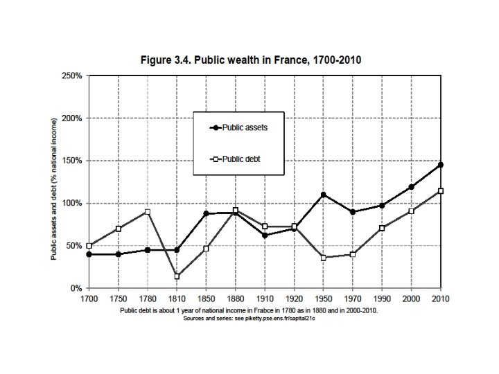
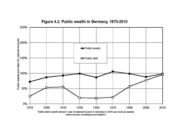
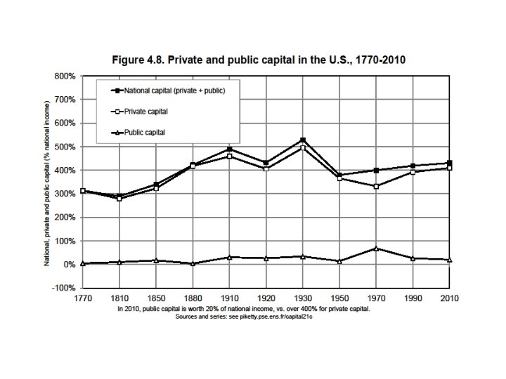
Private versus public wealth • National wealth Wn = Private wealth W + Public wealth Wg • Private wealth = private assets – private debt • Public wealth = public assets – public debt • Today, in most rich countries, public wealth close to 0 (public assets ≈ public debt ≈ 100% Y), and private wealth ≈ 95 -100% of national wealth • But it has not always been like this: sometime the govt owns a significant part of national wealth (2030% in 1950 s-60 s in W. Europe; 80% in USSR); sometime govt wealth<0 (huge debt), so that private wealth is significantly larger than national wealth

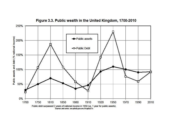
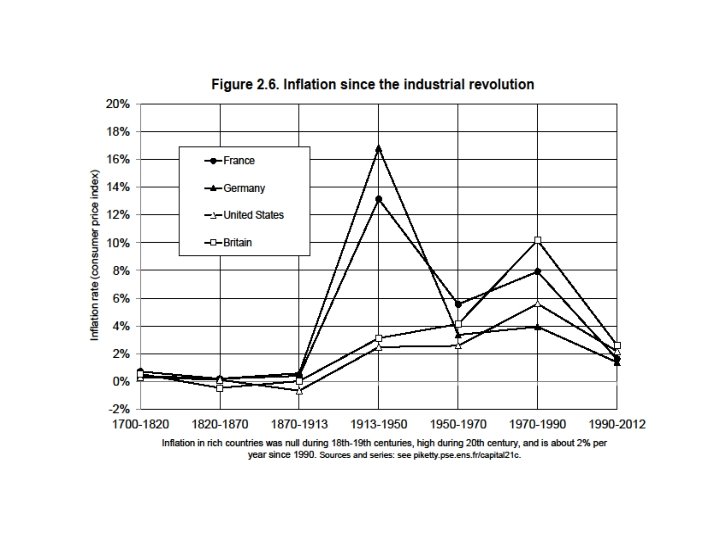
Britain: public debt and Ricardian equivalence • Britain = the country with the longest historical episodes of public debt: about 200% of Y around 18101820 (it took a century to reduce it below 50% by 1910, after a century of budget surpluses), and about 200% of Y again around 1950 (it was reduced faster, thanks to inflation) • Big difference with France (large inflation and/or repudiation during 1790 s & World Wars 1 and 2) and Germany (the country with the largest inflation in 1910 -1950, even excluding 1924) • Britain always paid back its debt (limited inflation, except 1950 -1980); this is why it took so long to reduce debt, especially during 19 c

War tributes, debt & state coercion • Rise of public debt in France 1815 -1880: war indemnities 1815 + « milliard des émigrés » 1825 (compensation to aristocrats for lost land rent during Revolution) + war tributes to Germany 1870 (about 30% Y in 1815 -1825 + 30% Y 1871=most of the rise) • War tributes are very common in history, particular in the context of colonial coercion: France and Spain against Morocco, Britain and France against China (see Truong 2015), etc. • 19 c = Gold standard = zero inflation: debt had to be repaid in full, so sacralization of public debt and private property had a real meaning • Most importantly, a country trying to default was immediately subject to military pressure, and sometime invasion = the standard justification for colonial expansion • 20 c = age of inflation and large debt repudiation • 21 c = back to 19 c sacralization of public debt & private property, but with economic/financial/legal threats rather than military?

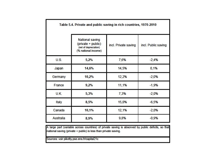
• Q. : What is the impact of public debt on capital accumulation? • A. : It depends on how the private saving responds to public deficit • National saving Sn = private saving S + public saving Sg (<0 if public deficit) • Suppose d. Sg<0 (public deficit↑) • If d. S=0 (no private saving response), then d. Sn<0 → decline in national wealth Wn : in effect public deficits absorb part of private saving (= « crowding out » ) • But if d. S>0, i. e. private saving increase in order to absorb the extra deficit, then crowding-out might be limited • In case d. S=-d. Sg, then d. Sn=0: national saving and national wealth are unaffected by public deficit • = apparently what happened in UK 1810 -1830: huge public debt, but no decline in private investment; extra private saving by British wealth holders, so that we observe a rise in private wealth, and no decline in national wealth = what Ricardo observes in 1817

• Key question: why was there no crowding out? • Barro 1974: in a representative agent model, rational agents should anticipate that they will pay more taxes in the future if today’s public deficit increase, so they save more in order to make reserves (for themselves or their successors) so as to pay these taxes in the future → the timing of taxes is irrelevant, « debt neutrality » (see also Barro 1987, Clark 2001) • Pb: the representative agent model does not make much sense to study these issues; in 19 c Britain, the agents holding public debt (=top 1% or top 10% wealth holders) are not the same as those paying taxes (=the entire population) • Public debt always involves large transfers between different social groups: for high wealth agents, it is better to lend money than to pay taxes… as long as the debt is paid back = big difference between 19 c and 20 c; will 21 c be more like 19 c, i. e. debt will be paid back? • Whether the Ricardian equivalence holds depends on the prosperity of private savers, the rate of return that they are being offered, the ability of the govt to convince them that they will be paid back; in 19 c UK, r was high, and govt highly credible

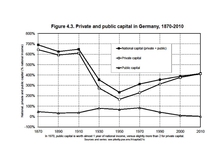
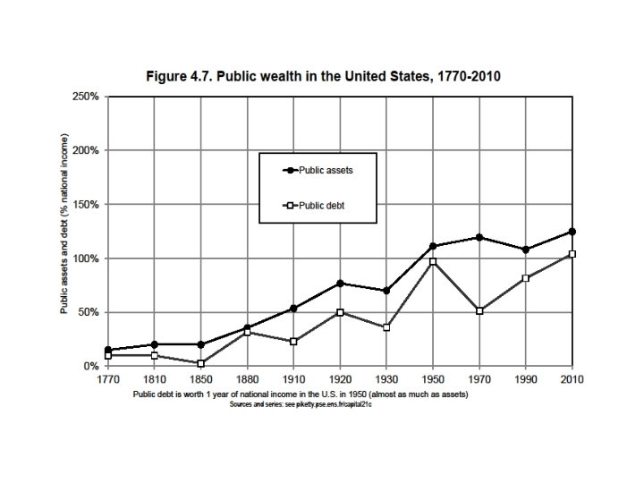
France: a mixed economy in 1950 -1980 • Historically, high public debt in France was always inflated away (more difficult with €) • In 1950, public debt<30% Y, and public assets >120% Y (public buildings + nationalized firms), so that net public wealth close to 100% Y; given that private wealth was close to 200% Y at that time, this means that in effect the govt owned about 1/3 of national wealth (and over 2/3 of large companies) • Same pattern in Germany 1950 (and Britain 1970) = the postwar mixed economy • Rise in public debt + privatization of public assets played a big role in rise of private wealth since 1980

Capital in Germany: stakeholder capitalism? • Same general pattern as in Britain and France • Except that NFA smaller in Germany in 18701910 (no colonial empire, late industrialization) • Except that the level of βn is lower in Germany during 1950 -2010 period: lower real estate prices (rent control, other regulations, geography? ), lower stock market prices (stakeholder capitalism? more on this later) • Except that NFA has been rising a lot in 1990 s 2000 s

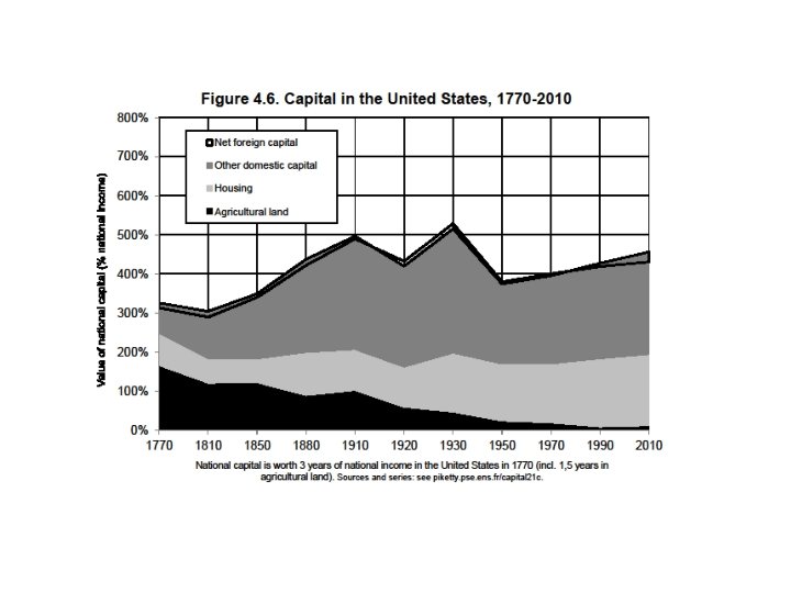
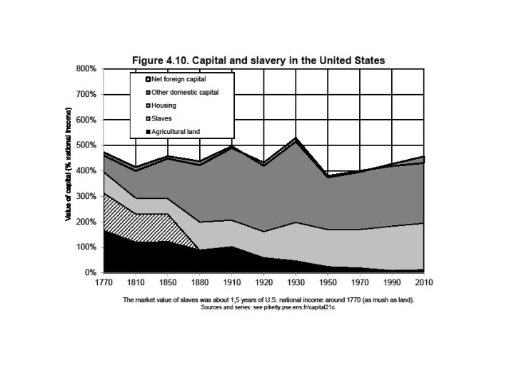
Capital in America: the role of slavery • Very different historical pattern than in Europe • Rising βn during 19 c, almost stable in 20 c • Level of βn generally smaller than in Europe, particularly in 19 c • Two factors: less time to accumulate capital; lower land price (more land in volume, but less land in value) • NFA always close to 0 in US; but <0 in Canada • Southern US before 1865: critical importance of slave capital in private wealth >> see lecture 5 (most extreme illustration of capital as power)

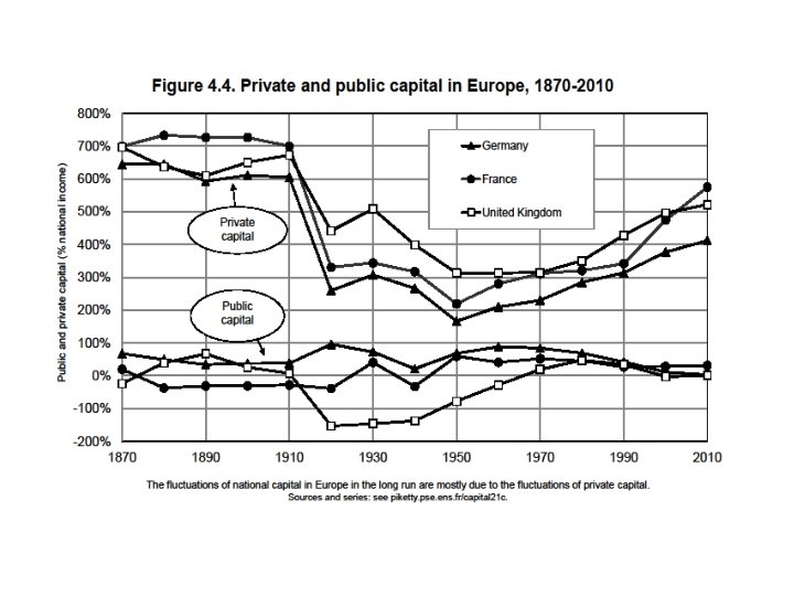
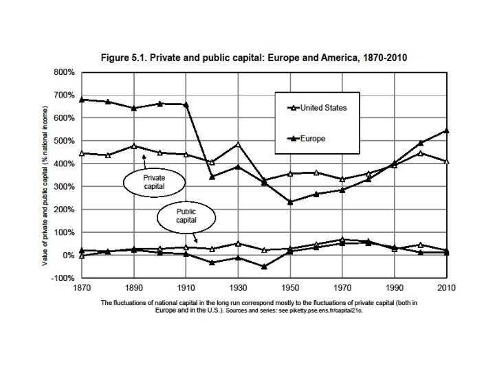
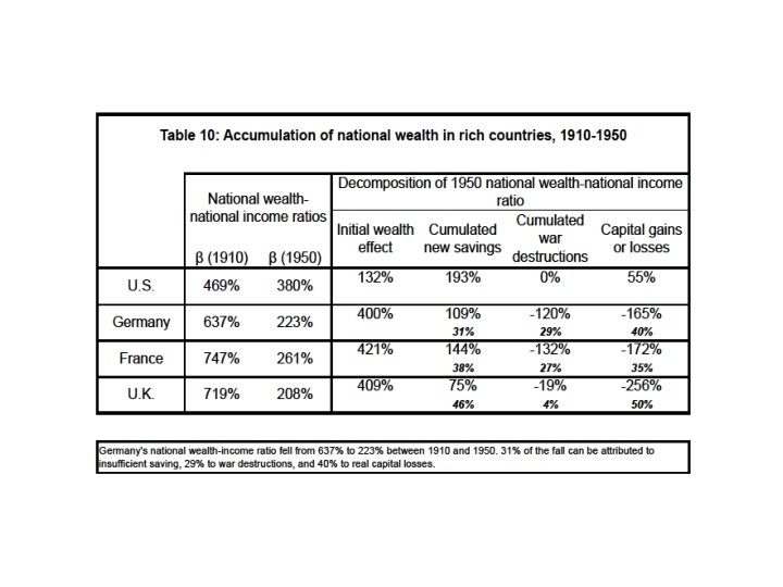
Summing up: what have we learned? • National wealth-income ratios βn=Wn/Y followed a large U-shaped curve in Europe: 600 -700% in 18 c-19 c until 1910, down to 200 -300% around 1950, back to 500 -600% in 2010 • U-shaped curve much less marked in the US • Most of the long run changes in βn are due to changes in the private wealth-income ratios β=W/Y • But changes in public wealth-income ratios βg=Wg/Y (>0 or <0) also played an important role (e. g. amplified the β decline between 1910 and 1950) • Changes in net foreign assets NFA (>0 or <0) also played an important role (e. g. account for a large part of the β decline between 1910 and 1950)

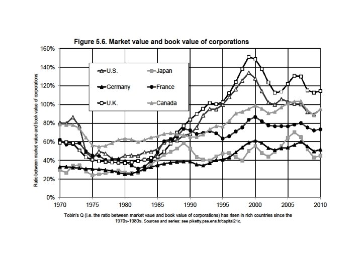
Market vs book value of corporations: capital and power • So far we used a market-value definition of national wealth Wn : corporations valued at stock market prices • Book value of corporations = assets – debt • Tobin’s Q ratio = (market value)/(book value) (>1 or <1) • Residual corporate wealth Wc = book value – market value • Book-value national wealth Wb = Wn + Wc • In principe, Q ≈ 1 (otherwise, investment should adjust), so that Wc ≈ 0 and Wb ≈ Wn • But Q can be systematically >1 if immaterial investment not well accounted in book assets • But Q can be systemativally <1 if shareholders have imperfect control of the firm (stakeholder model): this can explain why Q lower in Germany than in US-UK, and the general rise of Q since 1970 s-80 s

• Differences in legal systems, particularly in labor law & company law (stakeholder rights: “codetermination” = power sharing btw shareholders and workers) can explain different levels of Tobin’s Q • See Mc. Gaughey 2015 on corporate law & inequality; see also Mc. Gaughey 2015 & Schuster 2015 on codetermination in Germany, Sweden and other European countries : more codetermination → lower Tobin’s Q, but this can be good for the long-run investment of workers • Germany: employee representatives make 50% of supervisory board members (but shareholders have decisive vote and pick management board: German two-board system) • Sweden: 3 employees (≈30%) in single board of directors • France since 2013: 1 -2 employees (≈10 -20%) in board of directors • UK-US: 0 employee in board; shareholders have 100% of seats • One could also grant voting rights to workers in general shareholder meetings (Mc. Gaughey): economic democracy yet to be invented

Property regimes in history: from feudal to social • Feudal property involves various forms of « political » power over workers, e. g. judicial power, forced labor, etc. • French revolution: attempt to separate pure private property rights (legitimate) from political power (state monopoly). End of perpetual land rents. But in practice not easy to draw the line. • Blaufard, The Great Demarcation: the French Revolution and the Invention of Modern Property, OUP 2014. 1789: « abolition of feudal privileges » , but presumption that land rights are legitimate and need to be compensated. 1793: presumption that non-rent rights (e. g. selling rights) are feudal. 1815: compensation of aristocrats. In the end, church property was redistributed much more than aristocratic property. • Polanyi 1944: sacralisation of private property during 19 c led to 1914 -1945 shocks; after 1945, invention of new forms of social property: codetermination, mixed property, etc. • 21 c : social property still alive, but gradual return of a legal regime more favourable to private property rights

Intellectual property • One key shortcoming of existing balance sheets: intellectual property and immaterial capital (patents, copyrights, research, ideas, culture, . . ) are taken into account only when they are privately owned, so that a rise in wealth-income ratio might just reflect rising privatization of intellectual property & immaterial k • Major policy issues today: • How long should patents and copyrights last? • Is it possible to have private property rights on basic research articles that were publicly financed? • Is it possible to grant exclusivity rights for digitalization of works that are in public domain (library collections, art works, etc. )? • To what extent did weak IP laws in China and India facilitate world convergence? What would happened if all knowledge was privately owned through strong IP laws? • See e. g. Kapczynski 2015, « Intellectual Property & Inequality » ; Boyle 2003 « The Second Enclosure Movement and the Construction of the Public Domain » ; Kapczynski 2008 • See also Koh et al, « Labor Share Decline and the Capitalization of Intellectual Property Products » , WP 2015

Natural capital and land prices • Other key shortcoming of existing balance sheets: natural ressources (energy, forest, etc. ) are usually taken into account only when they are discovered and exploited; climate, air quality, etc. are never taken into account • Can depletion of natural capital (not to mention climate and other environmental damage be larger than the rise of private capital? • Natural capital depletion ≈ 3%-4% of Y at the world level, and 6%-8% Y in low income countries • This can largely undo the effect of positive net saving • See Barbier 2014 a, 2014 b • See also World Bank Wealth Accounting database • On common property ( « commons » ) and natural ressources management, see work by E. Olstrom • In the long run, changes in relative price of land other natural assets can be very important

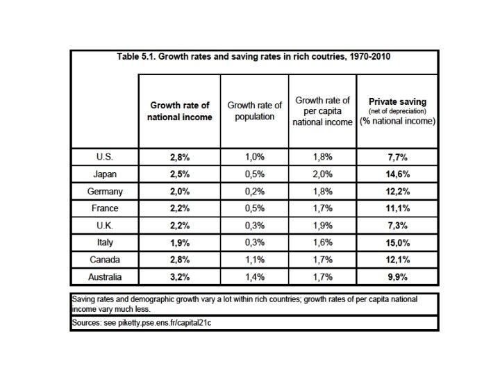
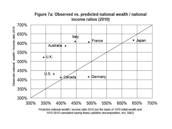
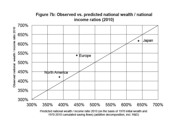
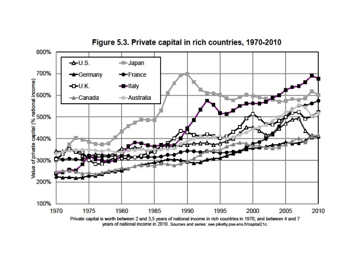
The rise of wealth-income ratios in rich countries : volume or price effects ? • Over 1970 -2010 period, the analysis can be extented to top 8 developed economies: US, Japan, Germany, France, UK, Italy, Canada, Australia (see Piketty-Zucman QJE 2014) • Around 1970, β≈200 -350% in all rich countries • Around 2010, β≈400 -700% in all rich countries • Asset price bubbles (real estate and/or stock market) are important in the short-run and medium-run • But the long-run evolution over 1970 -2010 is more than a bubble: it happens in every rich country, and can be partly explained by growth slowdown and the Harrod-Domar-Solow formula β=s/g (higher wealth-income ratio β if higher saving rate s and lower growth rate g) • It can also be explained by a structural price effect: rising land price, or rising power of owners, or rising domain of property?

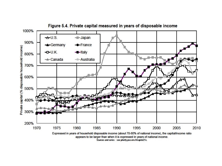
• The rise of β would be even larger is we were to divide private wealth W by disposable household income Yh rather than by national income Y • Yh used to be ≈90% of Y until early 20 c (=very low taxes and govt spendings); it is now ≈70 -80% of Y (=rise of in-kind transfers in education and healh) • βh=W/Yh is now as large as 800 -900% in some countries (Italy, Japan, France…) • But in order to make either cross-country or timeseries comparisons, it is better to use national income Y as a denominator (=more comprehensive and comparable income concept)

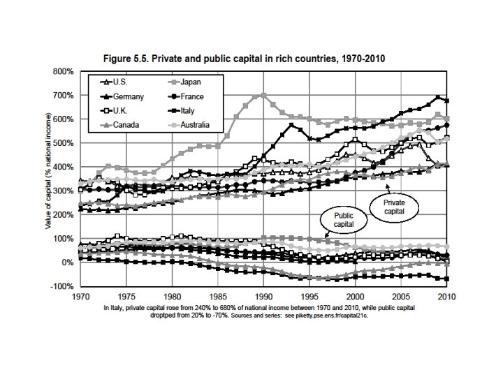
• 1970 -2010: rise of private wealth-income ratio β, decline in public wealth-inccome ratio βg • But the rise in β was much bigger than the decline in βg, so that national wealth-income ratio βn=β+βg rose substantially • Exemple: Italy. β rose from 240% to 680%, βg declined from 20% to -70%, so that βn rose from 260% to 610%. I. e. at most 1/4 of total increase in β can be attributed to a transfer from public to private wealth (privatisation and public debt).

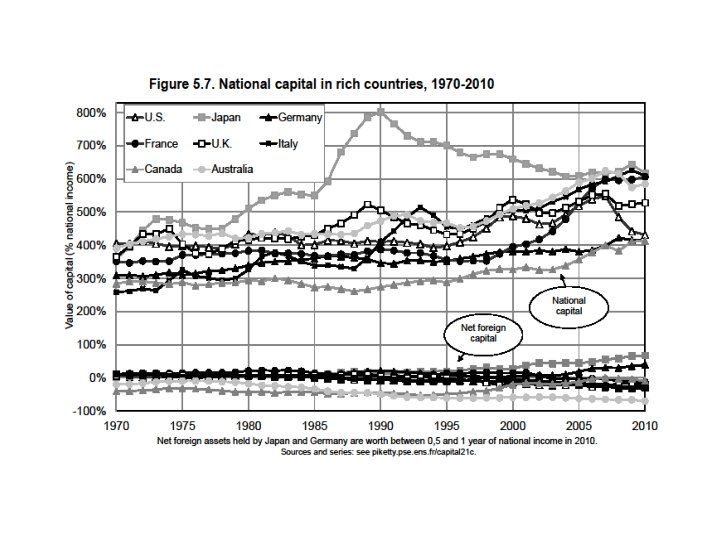
• In most countries, NFA ≈ 0, so rise in national wealth-income ratio ≈ rise in domestic capital-output ratio; in Japan and Germany, a non-trivial part of the rise in βn was invested abroad (≈ 1/4)

• Partial explanation for rise in wealth-income ratio in the very long run: growth slowdown and β = s/g (Harrod-Domar-Solow steady-state formula) • One-good capital accumulation model: Wt+1 = Wt + st. Yt → dividing both sides by Yt+1, we get: βt+1 = βt (1+gwt)/(1+gt) With 1+gwt = 1+st/βt = saving-induced wealth growth rate 1+gt = Yt+1/Yt = total income growth rate (productivity+population) • If saving rate st→ s and growth rate gt → g, then: βt → β = s/g • E. g. if s=10% & g=2%, then β = 500%: this is the only wealth-income ratio such that with s=10%, wealth rises at 2% per year, i. e. at the same pace as income • If s=10% and growth declines from g=3% to g=1, 5%, then the steadystate wealth-income ratio goes from about 300% to 600% → the large variations in growth rates and saving rates (g and s are determined by different factors and generally do not move together) explain the large variations in β over time and across countries (see Piketty-Zucman QJE 2014 & Course notes on wealth models)

• Two-good capital accumulation model: one capital good, one consumption good • Define 1+qt = real rate of capital gain (or capital loss) = excess of asset price inflation over consumer price inflation • Then βt+1 = βt (1+gwt)(1+qt)/(1+gt) With 1+gwt = 1+st/βt = saving-induced wealth growth rate 1+qt = capital-gains-induced wealth growth rate (=residual term) → Main finding: relative price effects (capital gains and losses) are key in the short and medium run and at local level; volume effects (saving and investment) are probably more important in the long run and at the national or continental level See the detailed decomposition results for wealth accumulation into volume and relative price effects in Piketty-Zucman, QJE 2014)

Can land housing prices also matter in the very long run? • Very difficult to identify pure land prices: hard to measure all past investment and improvment to land, the local infrastructures, etc. • There are good reasons to believe that price effects dominate in the short and medium run, but less so in the long run • However one can also find mechanims explaining why land housing prices might also matter in the very long run • See e. g Gyourko et al, « Superstar cities » , AEJ 2013 • See also Schularick et al 2015, « No price like home: global land prices 1870 -2012 » : the speed of technical progress in transportation technology has been relatively faster in 1850 -1960 than in 1960 -2010 (relative to other sectors such as biotech, computer, etc. ) (e. g. airplane speed unchanged in recent decades); this can potentially explain the rise of relative land prices in large capital cities in recent decades • More generally, in models with n goods, different speed of technical change can explain any long-run change in relative prices

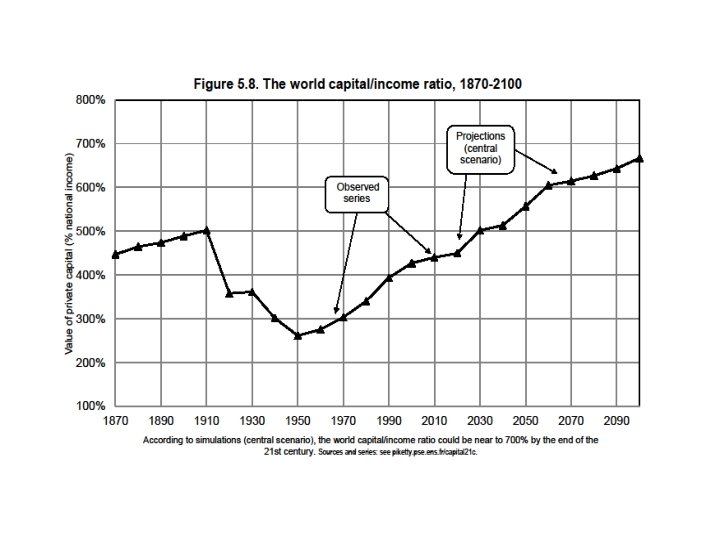
Capital in developing countries • Main lesson from historical experience of rich countries: wealth-income ratios β and βn have no reason to be stable over time and across countries • Unfortunately, limited balance sheet data for developing countries; key priority for future research: extending http: //www. wid. world/ to more countries • See simulations for world capital-income ratio in Capital…, chapter 5 & appendix tables • If global growth slowdown in the future (g≈1, 5%) and saving rates remain high (s≈10 -12%), then the global β might rise towards 700% (or more… or less…)

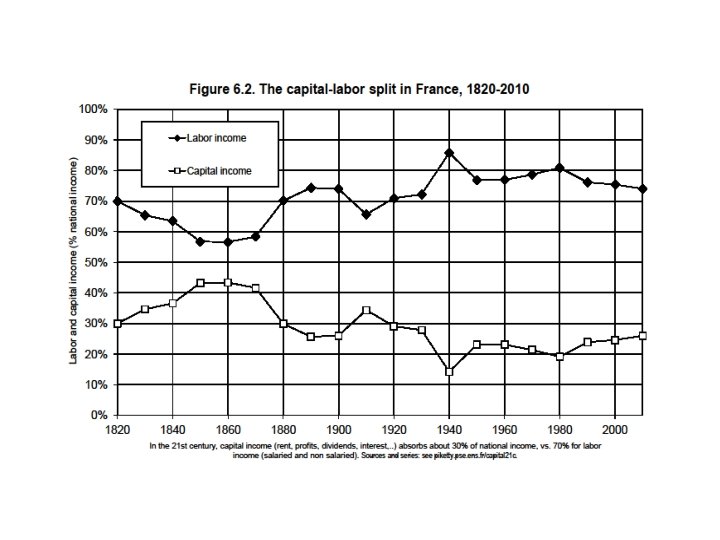
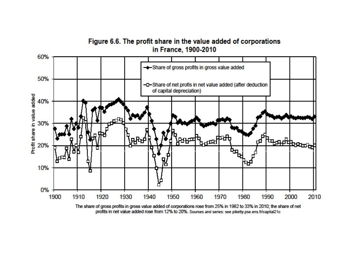
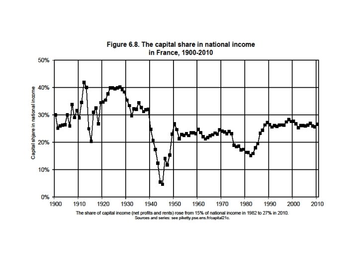
Capital-income ratios β vs. capital shares α • What are the consequences for the share α of capital income in national income? Not simple. Capital is multidimensional: legal system, relative prices and bargaining power matter a lot. One-sector production functions with perfect competition can be useful to think about some of the logical issues, but they are never the full story. • Capital/income ratio β=K/Y • Capital share α = YK/Y with YK = capital income (=sum of rent, dividends, interest, profits, etc. : i. e. all incomes going to the owners of capital, independently of any labor input) • I. e. β = ratio between capital stock and income flow • While α = share of capital income flow in total income flow • By definition: α = r x β With r = YK/K = average real rate of return to capital • If β=600% and r=5%, then α = 30% = typical values

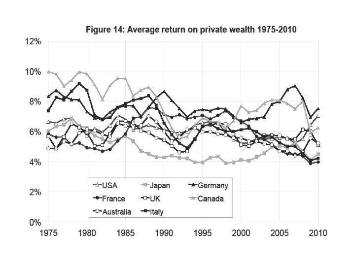
• In practice, the average rate of return to capital r (typically r≈4 -5%) varies a lot across assets and over individuals • Typically, rental return on housing = 3 -4% (i. e. the rental value of an appartment worth 100 000€ is generally about 3000 -4000€/year) (+ capital gain or loss) • Return on stock market (dividend + k gain) = as much as 6 -7% in the long run • Return on bank accounts or cash = as little as 1 -2% (but only a small fraction of total wealth) • Average return across all assets and individuals ≈ 4 -5%

The Cobb-Douglas production function • Cobb-Douglas production function: Y = F(K, L) = Kα L 1 -α • With perfect competition, wage rate v = marginal product of labor, rate of return r = marginal product of capital: r = FK = α Kα-1 L 1 -α and v = FL = (1 -α) Kα L-α • Therefore capital income YK = r K = α Y & labor income YL = v L = (1 -α) Y • I. e. capital & labor shares are entirely set by technology (say, α=30%, 1 -α=70%) and do not depend on quantities K, L • Intuition: Cobb-Douglas ↔ elasticity of substitution between K & L is exactly equal to 1 • I. e. if v/r rises by 1%, K/L=α/(1 -α) v/r also rises by 1%. So the quantity response exactly offsets the change in prices: if wages ↑by 1%, then firms use 1% less labor, so that labor share in total output remains the same as before

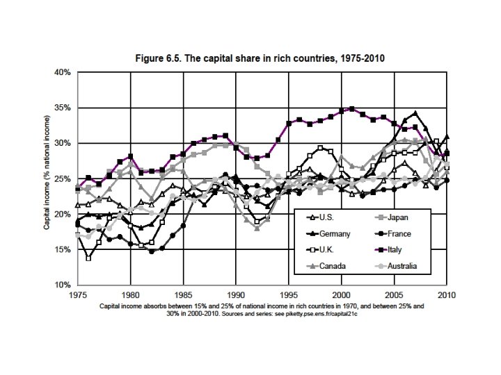
The limits of Cobb-Douglas • Economists like Cobb-Douglas production function, because they like simple stories, and because capital shares sometime seem to be approximately stable • However it is only an approximation: in practice, capital shares α vary in the 20 -40% range over time and between countries (or even sometime in the 10 -50% range) • In 19 c, capital shares were closer to 40%; in 20 c, they were closer to 20 -30%; structural rise of human capital (i. e. exponent α↓ in Cobb-Douglas production function Y = Kα L 1 -α ? ), or purely temporary phenomenon ? • Over 1970 -2010 period, capital shares have increased from 1525% to 25 -30% in rich countries : very difficult to explain with Cobb-Douglas framework

The CES production function • CES = a simple way to think about changing capital shares • CES : Y = F(K, L) = [a K(σ-1)/σ + b L(σ-1)/σ ]σ/(σ-1) with a, b = constant σ = constant elasticity of substitution between K and L • σ →∞: linear production function Y = r K + v L (infinite substitution: machines can replace workers and vice versa, so that the returns to capital and labor do not fall at all when the quantity of capital or labor rise) ( = robot economy) • σ → 0: F(K, L)=min(r. K, v. L) (fixed coefficients) = no substitution possibility: one needs exactly one machine per worker • σ → 1: converges toward Cobb-Douglas; but all intermediate cases are also possible: Cobb-Douglas is just one possibility among many • Compute the first derivative r = FK : the marginal product to capital is given by r = FK = a β-1/σ (with β=K/Y) I. e. r ↓ as β↑ (more capital makes capital less useful), but the important point is that the speed at which r ↓ depends on σ

• With r = FK = a β-1/σ, the capital share α is given by: α = r β = a β(σ-1)/σ • I. e. α is an increasing function of β if and only if σ>1 (and stable iff σ=1) • The important point is that with large changes in the volume of capital β, small departures from σ=1 are enough to explain large changes in α • If σ = 1. 5, capital share rises from α=28% to α =36% when β rises from β=250% to β =500% = more or less what happened since the 1970 s • In case β reaches β =800%, α would reach α =42% • In case σ =1. 8, α would be as large as α =53%

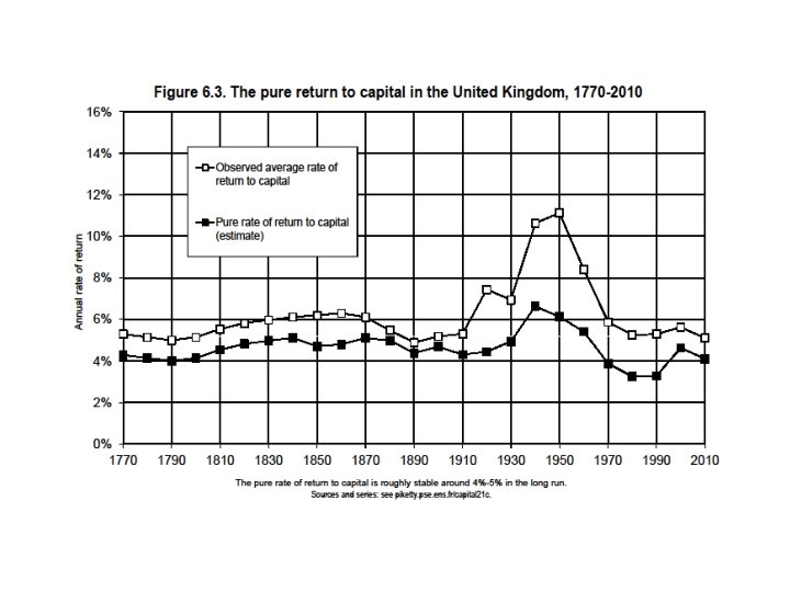
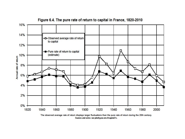
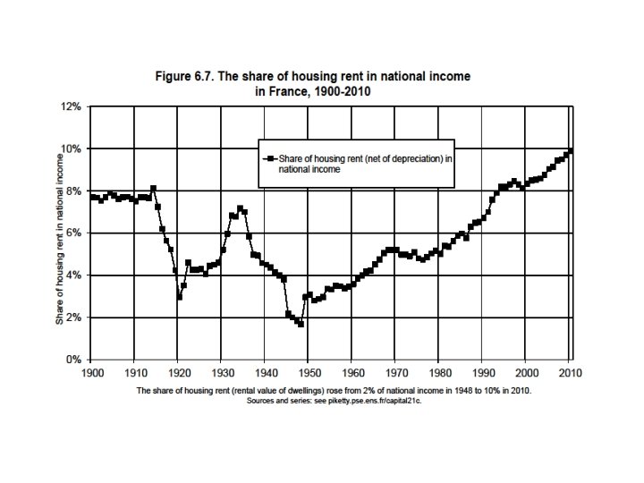
Measurement problems with capital shares • In many ways, β is easier to measure than α • In principle, capital income = all income flows going to capital owners (independanty of any labor input); labor income = income flows going to labor earners (independantly of any capital input) • But in practice, the line is often hard to draw: family firms, selfsemployed workers, informal financial intermediation costs (=the time spent to manage one’s own portfolio) • If one measures the capital share α from national accounts (rent+dividend+interest+profits) and compute average return r=α/β, then the implied r often looks very high for a pure return to capital ownership: it probably includes a non-negligible entrepreneurial labor component, particularly in reconstruction periods with low β and high r; the pure return might be 20 -30% smaller (see estimates) • One should use two-sector models Y=q. Yh+Yb (housing + business; q = relative housing price); return to housing = closer to pure return to capital (or n-sector models)

Recent work on capital shares • Imperfect competition and globalization: see Karabarmounis. Neiman 2013 , « The Global Decline in the Labor Share » ; see also Karabarmounis-Neiman 2014; Assous-Dutt 2013, Dutt 2015 • Multi-sector models. Atkinson-Summers: Y=F(K 1, AL+BK 2) • Public vs private firms: see Azmat-Manning-Van Reenen 2011, « Privatization and the Decline of the Labor Share in GDP: A Cross. Country Aanalysis of the Network Industries » • K shares and CEO pay : see Pursey 2013, «CEO Pay and Factor shares: Bargaining effects in US corporations 1970 -2011 » • Capital shares in developing countries: under-studied issue • Capital share α is often v. high in poor countries (40 -50% instead of 20 -30%), but why: low bargaining power of labor, and/or natural ressources, and/or measurement pb? Lots of missing data; see e. g. ILO Global Wage Report 2014 -15