Dynamic Programming Dynamic Programming is a general algorithm

Dynamic Programming .

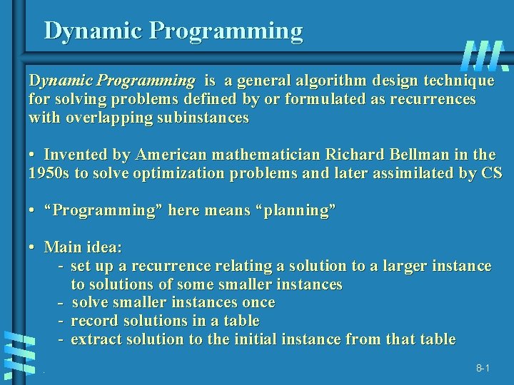
Dynamic Programming is a general algorithm design technique for solving problems defined by or formulated as recurrences with overlapping subinstances • Invented by American mathematician Richard Bellman in the 1950 s to solve optimization problems and later assimilated by CS • “Programming” here means “planning” • Main idea: - set up a recurrence relating a solution to a larger instance to solutions of some smaller instances - solve smaller instances once - record solutions in a table - extract solution to the initial instance from that table. 8 -1

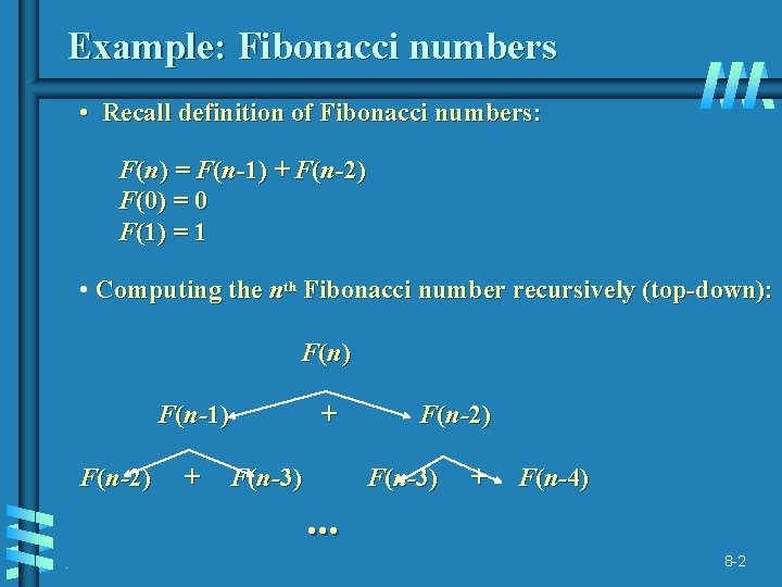
Example: Fibonacci numbers • Recall definition of Fibonacci numbers: F(n) = F(n-1) + F(n-2) F(0) = 0 F(1) = 1 • Computing the nth Fibonacci number recursively (top-down): F (n ) F(n-1) F(n-2) + + F(n-3) F(n-2) F(n-3) + F(n-4) . . 8 -2

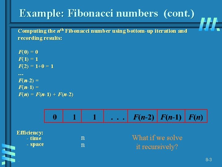
Example: Fibonacci numbers (cont. ) Computing the nth Fibonacci number using bottom-up iteration and recording results: F(0) = 0 F(1) = 1 F(2) = 1+0 = 1 … F(n-2) = F(n-1) + F(n-2) Efficiency: - time - space. n n What if we solve it recursively? 8 -3

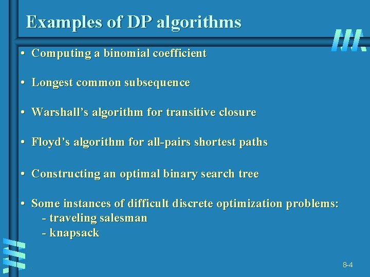
Examples of DP algorithms • Computing a binomial coefficient • Longest common subsequence • Warshall’s algorithm for transitive closure • Floyd’s algorithm for all-pairs shortest paths • Constructing an optimal binary search tree • Some instances of difficult discrete optimization problems: - traveling salesman - knapsack. 8 -4

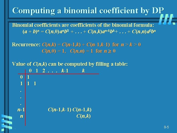
Computing a binomial coefficient by DP Binomial coefficients are coefficients of the binomial formula: (a + b)n = C(n, 0)anb 0 +. . . + C(n, k)an-kbk +. . . + C(n, n)a 0 bn Recurrence: C(n, k) = C(n-1, k) + C(n-1, k-1) for n > k > 0 C(n, 0) = 1, C(n, n) = 1 for n 0 Value of C(n, k) can be computed by filling a table: 0 1 2. . . k-1 k 0 1 1. . . n-1 C(n-1, k-1) C(n-1, k) n C(n, k). 8 -5

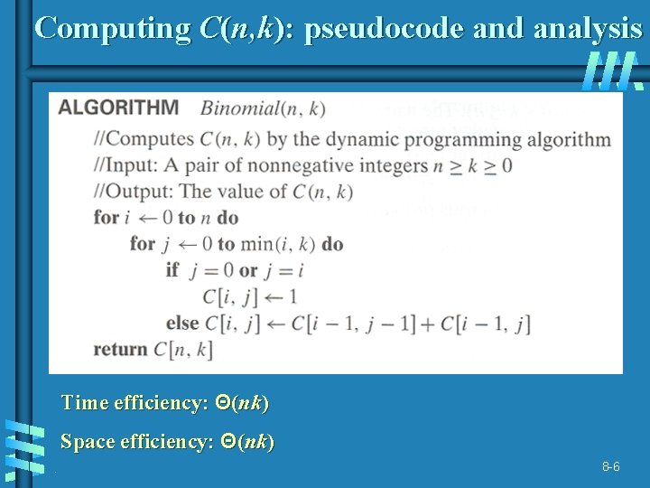
Computing C(n, k): pseudocode and analysis Time efficiency: Θ(nk) Space efficiency: Θ(nk). 8 -6

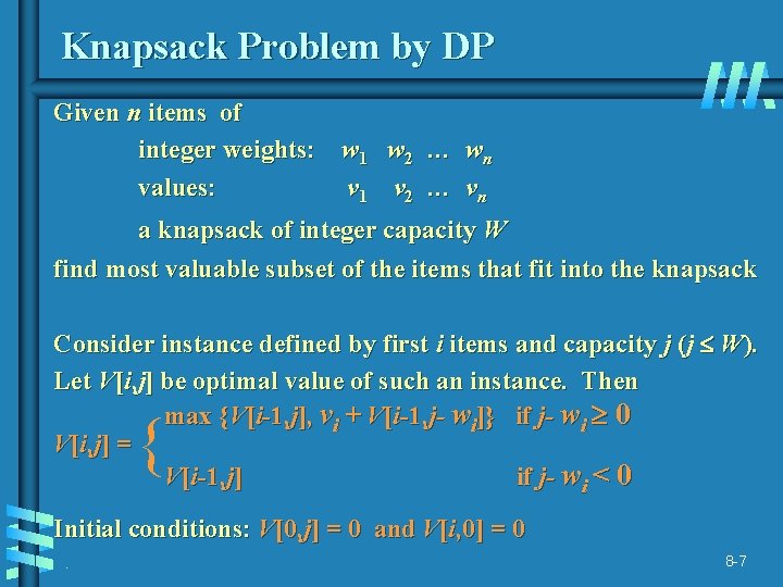
Knapsack Problem by DP Given n items of integer weights: w 1 w 2 … wn values: v 1 v 2 … vn a knapsack of integer capacity W find most valuable subset of the items that fit into the knapsack Consider instance defined by first i items and capacity j (j W). Let V[i, j] be optimal value of such an instance. Then max {V[i-1, j], vi + V[i-1, j- wi]} if j- wi 0 V[i, j] = V[i-1, j] if j- wi < 0 { Initial conditions: V[0, j] = 0 and V[i, 0] = 0. 8 -7

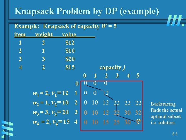
Knapsack Problem by DP (example) Example: Knapsack of capacity W = 5 item weight value 1 2 $12 2 1 $10 3 3 $20 4 2 $15 capacity j 0 1 2 3 4 0 0 5 w 1 = 2, v 1= 12 1 0 0 12 w 2 = 1, v 2= 10 2 0 10 12 22 22 22 w 3 = 3, v 3= 20 3 0 10 12 22 30 32 w 4 = 2, v 4= 15 4 0 10 15 25 30 37 ? . Backtracing finds the actual optimal subset, i. e. solution. 8 -8

Knapsack Problem by DP (pseudocode) Algorithm DPKnapsack(w[1. . n], v[1. . n], W) var V[0. . n, 0. . W], P[1. . n, 1. . W]: int for j : = 0 to W do V[0, j] : = 0 for i : = 0 to n do Running time and space: O(n. W). V[i, 0] : = 0 for i : = 1 to n do for j : = 1 to W do if w[i] j and v[i] + V[i-1, j-w[i]] > V[i-1, j] then V[i, j] : = v[i] + V[i-1, j-w[i]]; P[i, j] : = j-w[i] else V[i, j] : = V[i-1, j]; P[i, j] : = j return V[n, W] and the optimal subset by backtracing. 8 -9

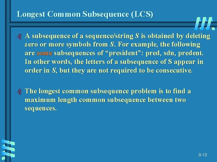
Longest Common Subsequence (LCS) b A subsequence of a sequence/string S is obtained by deleting zero or more symbols from S. For example, the following are some subsequences of “president”: pred, sdn, predent. In other words, the letters of a subsequence of S appear in order in S, but they are not required to be consecutive. b The longest common subsequence problem is to find a maximum length common subsequence between two sequences. . 8 -10

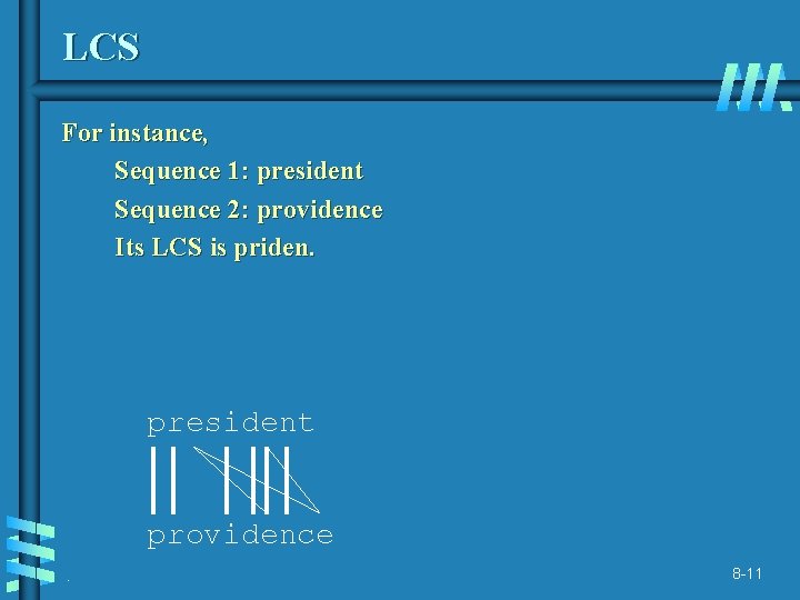
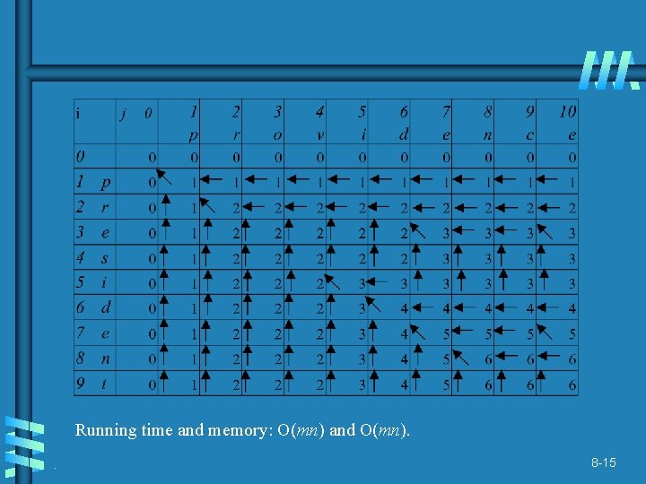
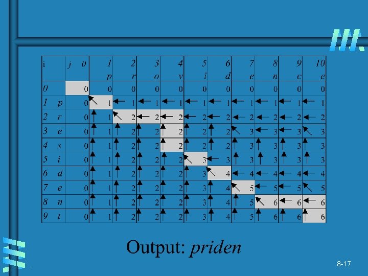
LCS For instance, Sequence 1: president Sequence 2: providence Its LCS is priden. president providence. 8 -11

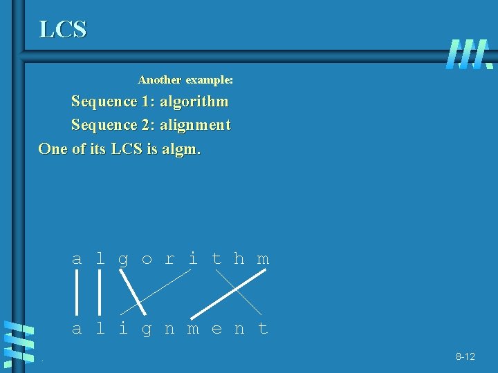
LCS Another example: Sequence 1: algorithm Sequence 2: alignment One of its LCS is algm. a l g o r i t h m a l i g n m e n t. 8 -12

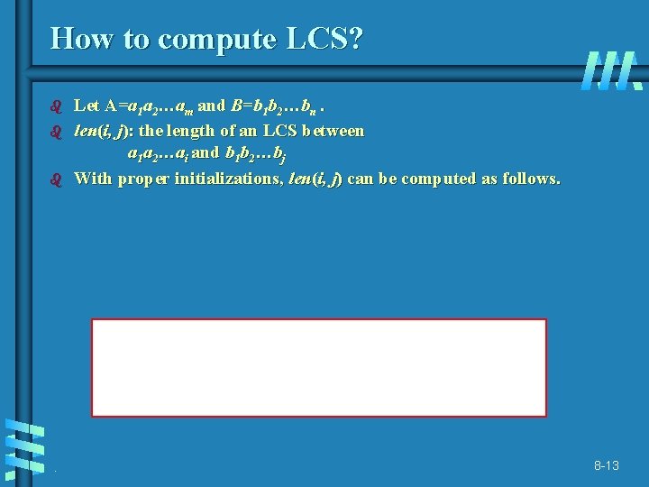
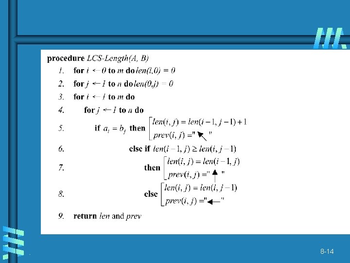
How to compute LCS? b b b . Let A=a 1 a 2…am and B=b 1 b 2…bn. len(i, j): the length of an LCS between a 1 a 2…ai and b 1 b 2…bj With proper initializations, len(i, j) can be computed as follows. 8 -13

. 8 -14

Running time and memory: O(mn) and O(mn). . 8 -15

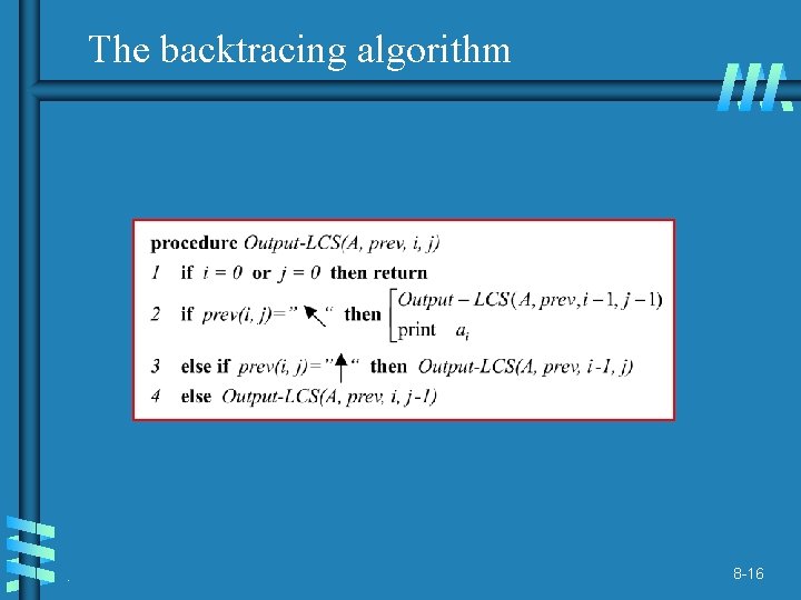
The backtracing algorithm . 8 -16

. 8 -17

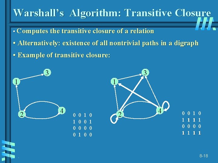
Warshall’s Algorithm: Transitive Closure • Computes the transitive closure of a relation • Alternatively: existence of all nontrivial paths in a digraph • Example of transitive closure: 3 3 1 1 2 . 4 0 1 0 0 0 1 1 0 0 2 4 0 1 0 1 1 1 0 1 0 1 8 -18

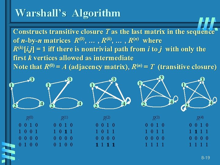
Warshall’s Algorithm Constructs transitive closure T as the last matrix in the sequence of n-by-n matrices R(0), … , R(k), … , R(n) where R(k)[i, j] = 1 iff there is nontrivial path from i to j with only the first k vertices allowed as intermediate Note that R(0) = A (adjacency matrix), R(n) = T (transitive closure) 3 1 1 4 2 0 1 0 0. R(0) 0 1 0 3 0 1 0 0 1 4 2 0 1 0 0 R(1) 0 1 0 0 3 0 1 1 4 2 R(2) 0 1 0 0 1 1 0 1 3 3 1 4 2 0 1 R(3) 0 1 0 0 1 1 0 1 4 2 0 1 R(4) 0 1 1 1 0 0 1 1 0 1 8 -19

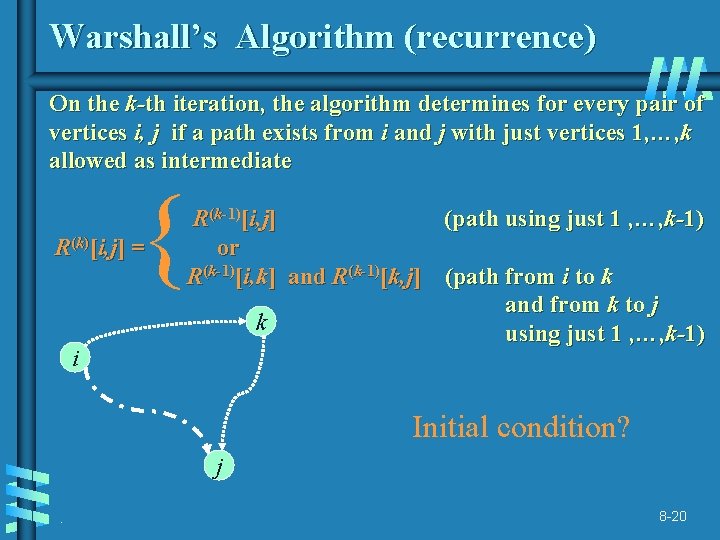
Warshall’s Algorithm (recurrence) On the k-th iteration, the algorithm determines for every pair of vertices i, j if a path exists from i and j with just vertices 1, …, k allowed as intermediate { R(k)[i, j] = i R(k-1)[i, j] (path using just 1 , …, k-1) or R(k-1)[i, k] and R(k-1)[k, j] (path from i to k and from k to j k using just 1 , …, k-1) Initial condition? j. 8 -20

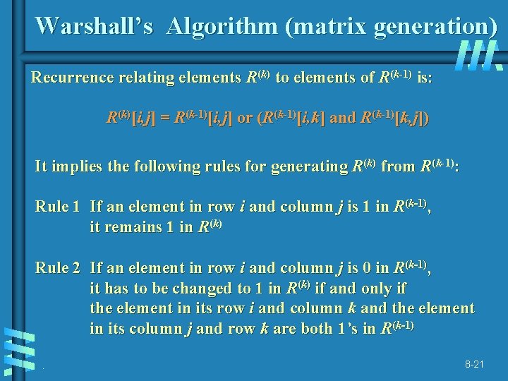
Warshall’s Algorithm (matrix generation) Recurrence relating elements R(k) to elements of R(k-1) is: R(k)[i, j] = R(k-1)[i, j] or (R(k-1)[i, k] and R(k-1)[k, j]) It implies the following rules for generating R(k) from R(k-1): Rule 1 If an element in row i and column j is 1 in R(k-1), it remains 1 in R(k) Rule 2 If an element in row i and column j is 0 in R(k-1), it has to be changed to 1 in R(k) if and only if the element in its row i and column k and the element in its column j and row k are both 1’s in R(k-1). 8 -21

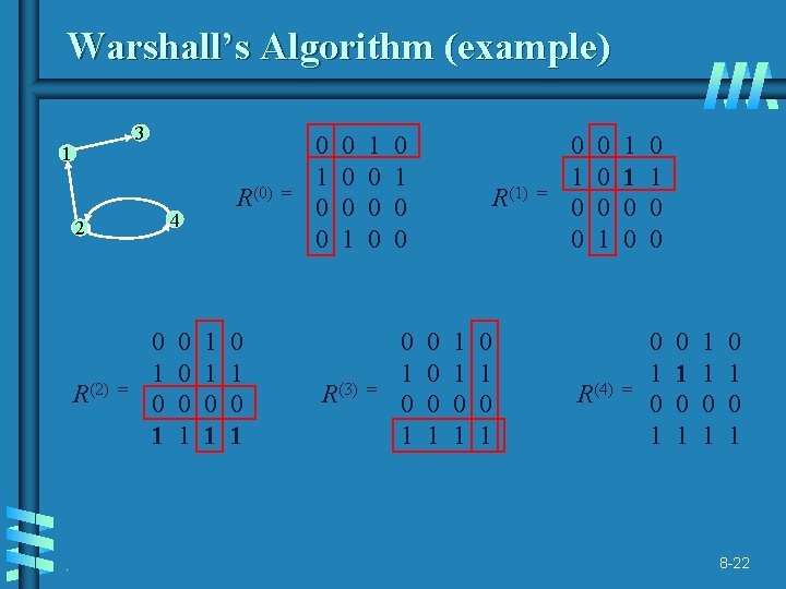
Warshall’s Algorithm (example) 3 1 4 2 R(2) . R(0) = 0 1 0 0 0 1 1 1 0 1 0 1 = 0 1 0 0 0 1 R(3) 1 0 0 0 = 0 1 0 0 0 1 R(1) 0 0 0 1 1 1 0 1 0 1 = 0 1 0 0 0 1 R(4) 1 1 0 0 0 1 0 0 = 0 1 0 1 1 1 0 1 0 1 8 -22

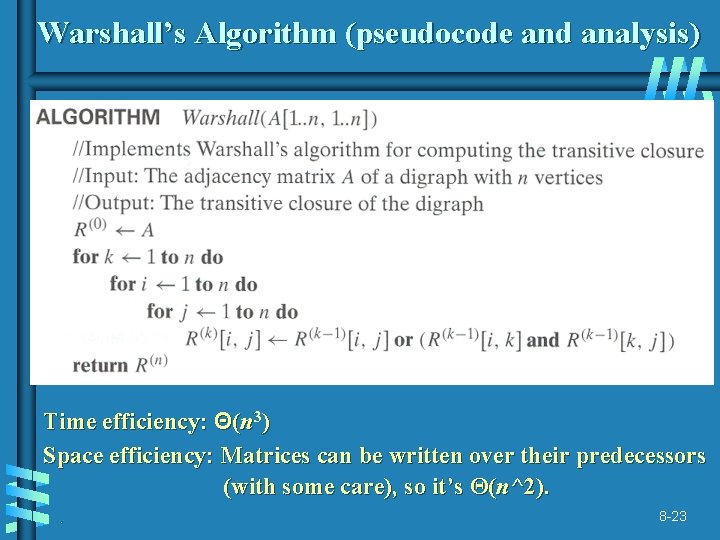
Warshall’s Algorithm (pseudocode and analysis) Time efficiency: Θ(n 3) Space efficiency: Matrices can be written over their predecessors (with some care), so it’s Θ(n^2). . 8 -23

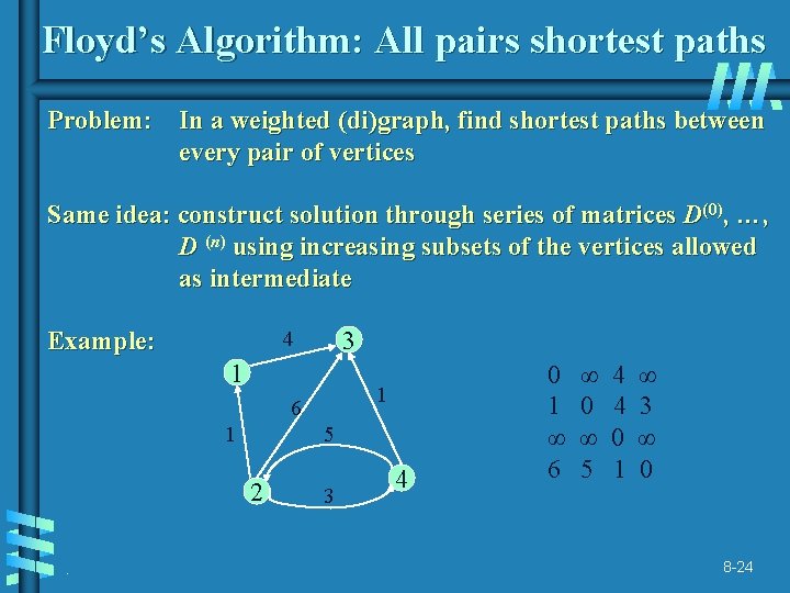
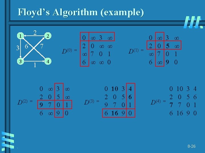
Floyd’s Algorithm: All pairs shortest paths Problem: In a weighted (di)graph, find shortest paths between every pair of vertices Same idea: construct solution through series of matrices D(0), …, D (n) using increasing subsets of the vertices allowed as intermediate Example: 3 4 1 1 6 1 5 2. 3 4 0 1 ∞ 6 ∞ 0 ∞ 5 4 4 0 1 ∞ 3 ∞ 0 8 -24

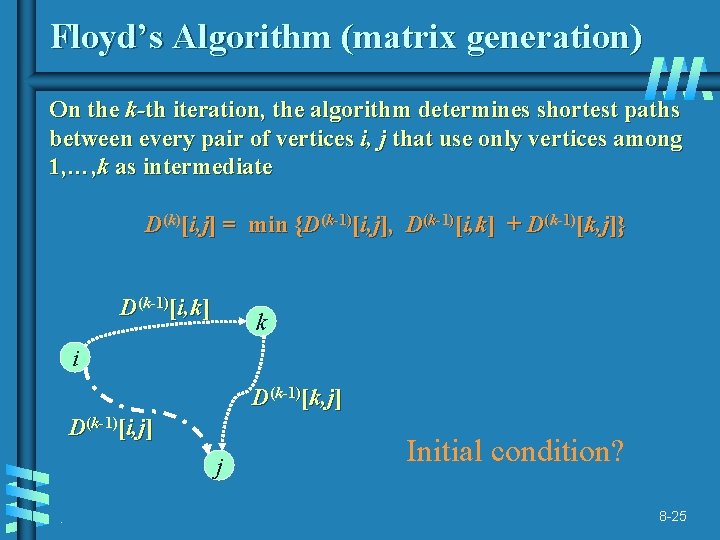
Floyd’s Algorithm (matrix generation) On the k-th iteration, the algorithm determines shortest paths between every pair of vertices i, j that use only vertices among 1, …, k as intermediate D(k)[i, j] = min {D(k-1)[i, j], D(k-1)[i, k] + D(k-1)[k, j]} D(k-1)[i, k] k i D(k-1)[k, j] D(k-1)[i, j] j. Initial condition? 8 -25

Floyd’s Algorithm (example) 2 1 3 6 7 3 D(2) . 2 4 1 = D(0) 0 2 9 6 ∞ 0 7 ∞ 3 5 0 9 ∞ ∞ 1 0 = 0 2 ∞ 6 ∞ 0 7 ∞ D(3) 3 ∞ 0 ∞ = ∞ ∞ 1 0 0 2 9 6 10 0 7 16 D(1) 3 5 0 9 4 6 1 0 = 0 2 ∞ 6 ∞ 0 7 ∞ D(4) 3 5 0 9 = ∞ ∞ 1 0 0 2 7 6 10 0 7 16 3 5 0 9 4 6 1 0 8 -26

Floyd’s Algorithm (pseudocode and analysis) If D[i, k] + D[k, j] < D[i, j] then P[i, j] k Time efficiency: Θ(n 3) Since the superscripts k or k-1 make no difference to D[i, k] and D[k, j]. Space efficiency: Matrices can be written over their predecessors Note: Works on graphs with negative edges but without negative cycles. Shortest paths themselves can be found, too. How? . 8 -27

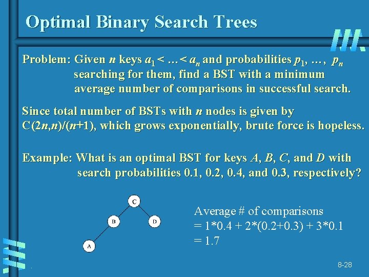
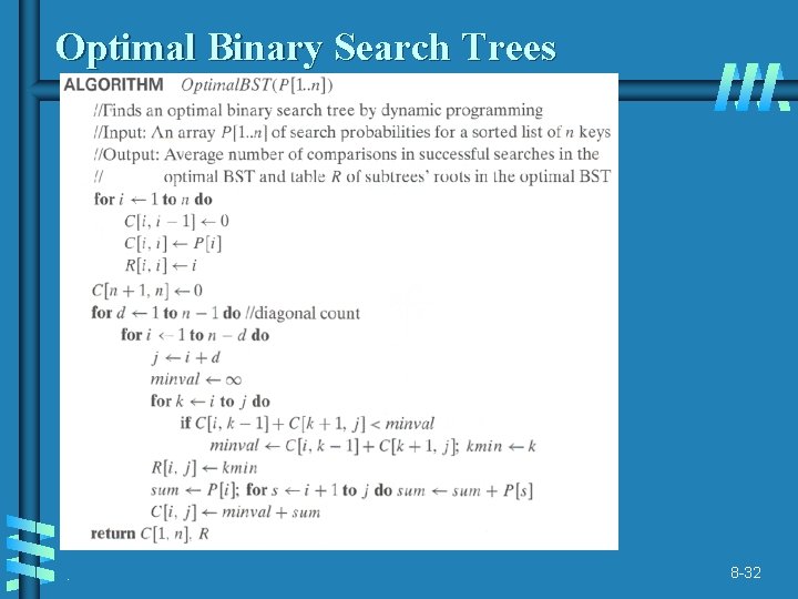
Optimal Binary Search Trees Problem: Given n keys a 1 < …< an and probabilities p 1, …, pn searching for them, find a BST with a minimum average number of comparisons in successful search. Since total number of BSTs with n nodes is given by C(2 n, n)/(n+1), which grows exponentially, brute force is hopeless. Example: What is an optimal BST for keys A, B, C, and D with search probabilities 0. 1, 0. 2, 0. 4, and 0. 3, respectively? Average # of comparisons = 1*0. 4 + 2*(0. 2+0. 3) + 3*0. 1 = 1. 7. 8 -28

DP for Optimal BST Problem Let C[i, j] be minimum average number of comparisons made in T[i, j], optimal BST for keys ai < …< aj , where 1 ≤ i ≤ j ≤ n. Consider optimal BST among all BSTs with some ak (i ≤ k ≤ j ) as their root; T[i, j] is the best among them. C[i, j] = min {pk · 1 + i≤k≤j k-1 ∑ ps (level as in T[i, k-1] +1) + s=i j ∑ ps (level as in T[k+1, j] +1)} s =k+1. 8 -29

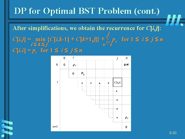
DP for Optimal BST Problem (cont. ) After simplifications, we obtain the recurrence for C[i, j]: j C[i, j] = min {C[i, k-1] + C[k+1, j]} + ∑ ps for 1 ≤ i ≤ j ≤ n i≤k≤j C[i, i] = pi for 1 ≤ i ≤ j ≤ n . s=i 8 -30

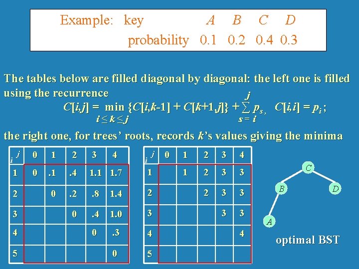
Example: key A B C D probability 0. 1 0. 2 0. 4 0. 3 The tables below are filled diagonal by diagonal: the left one is filled using the recurrence j C[i, j] = min {C[i, k-1] + C[k+1, j]} + ∑ ps , C[i, i] = pi ; i≤k≤j s=i the right one, for trees’ roots, records k’s values giving the minima j 0 1 2 3 1 0 . 1 . 4 1. 1 1. 7 1 0 . 2 . 8 1. 4 2 0 . 4 1. 0 3 0 . 3 4 0 5 i 2 3 4 5 4 i j 0 1 2 3 4 1 2 3 3 3 3 4 C B D A optimal BST

Optimal Binary Search Trees . 8 -32

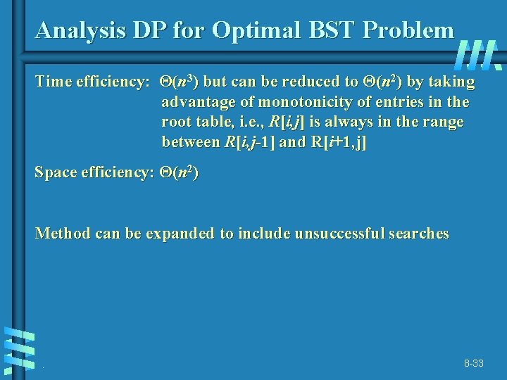
Analysis DP for Optimal BST Problem Time efficiency: Θ(n 3) but can be reduced to Θ(n 2) by taking advantage of monotonicity of entries in the root table, i. e. , R[i, j] is always in the range between R[i, j-1] and R[i+1, j] Space efficiency: Θ(n 2) Method can be expanded to include unsuccessful searches . 8 -33