Dynamic Programming Dynamic Programming is a general algorithm

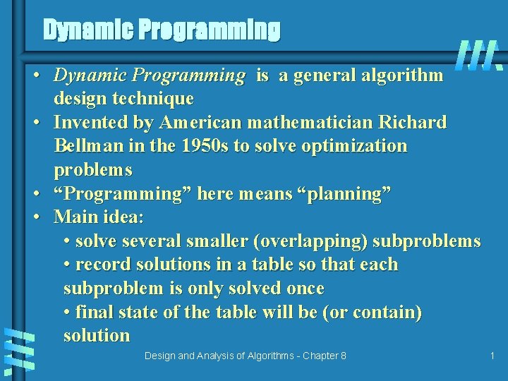
Dynamic Programming • Dynamic Programming is a general algorithm design technique • Invented by American mathematician Richard Bellman in the 1950 s to solve optimization problems • “Programming” here means “planning” • Main idea: • solve several smaller (overlapping) subproblems • record solutions in a table so that each subproblem is only solved once • final state of the table will be (or contain) solution Design and Analysis of Algorithms - Chapter 8 1

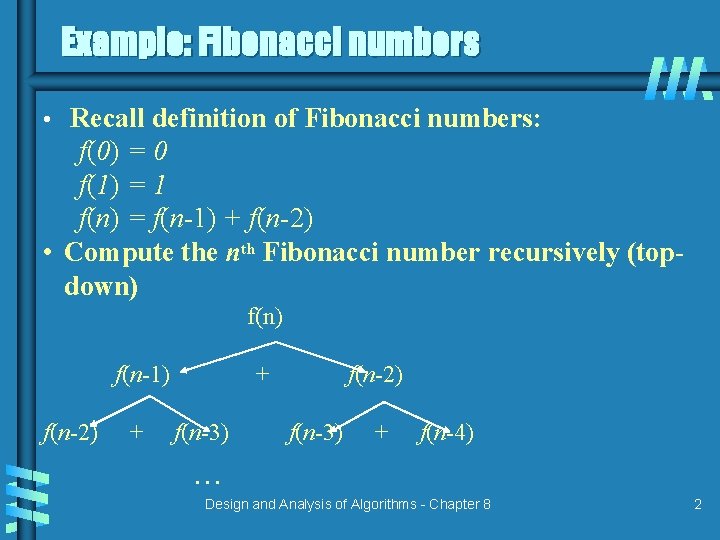
Example: Fibonacci numbers • Recall definition of Fibonacci numbers: f(0) = 0 f(1) = 1 f(n) = f(n-1) + f(n-2) • Compute the nth Fibonacci number recursively (topdown) f(n-1) f(n-2) + + f(n-3) f(n-2) f(n-3) + f(n-4) . . . Design and Analysis of Algorithms - Chapter 8 2

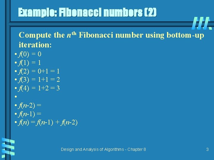
Example: Fibonacci numbers (2) Compute the nth Fibonacci number using bottom-up iteration: • f(0) = 0 • f(1) = 1 • f(2) = 0+1 = 1 • f(3) = 1+1 = 2 • f(4) = 1+2 = 3 • • f(n-2) = • f(n-1) = • f(n) = f(n-1) + f(n-2) Design and Analysis of Algorithms - Chapter 8 3

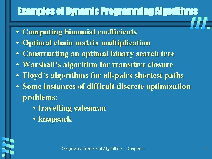
Examples of Dynamic Programming Algorithms • • • Computing binomial coefficients Optimal chain matrix multiplication Constructing an optimal binary search tree Warshall’s algorithm for transitive closure Floyd’s algorithms for all-pairs shortest paths Some instances of difficult discrete optimization problems: • travelling salesman • knapsack Design and Analysis of Algorithms - Chapter 8 4

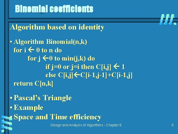
Binomial coefficients Algorithm based on identity • Algorithm Binomial(n, k) for i 0 to n do for j 0 to min(j, k) do if j=0 or j=i then C[i, j] 1 else C[i, j] C[i-1, j-1]+C[i-1, j] return C[n, k] • Pascal’s Triangle • Example • Space and Time efficiency Design and Analysis of Algorithms - Chapter 8 5

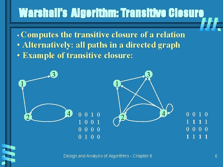
Warshall’s Algorithm: Transitive Closure • Computes the transitive closure of a relation • Alternatively: all paths in a directed graph • Example of transitive closure: 3 3 1 1 2 4 0 1 0 0 0 1 1 0 0 2 Design and Analysis of Algorithms - Chapter 8 4 0 1 0 1 1 1 0 1 0 1 6

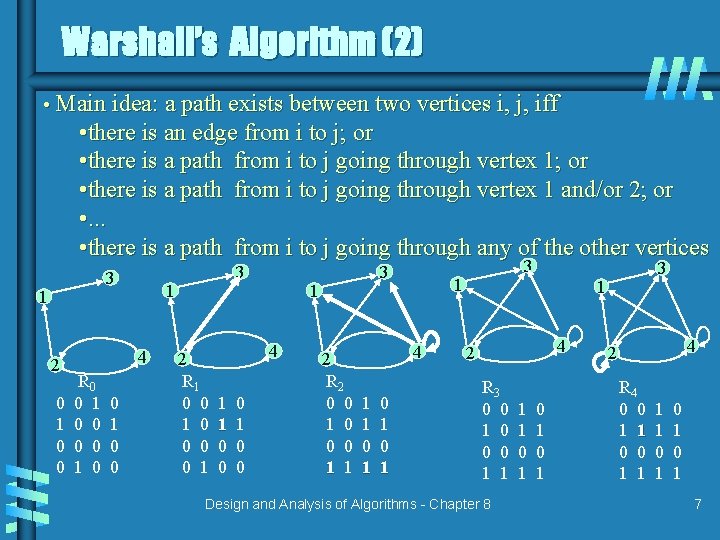
Warshall’s Algorithm (2) • Main idea: a path exists between two vertices i, j, iff • there is an edge from i to j; or • there is a path from i to j going through vertex 1 and/or 2; or • . . . • there is a path from i to j going through any of the other vertices 3 1 2 0 1 0 0 1 4 R 0 0 1 0 0 3 2 R 1 0 0 0 0 1 1 4 1 1 0 0 0 1 0 0 3 2 R 2 0 0 1 0 0 0 1 1 1 4 1 1 0 1 0 1 3 3 1 4 2 R 3 0 0 1 0 0 0 1 1 Design and Analysis of Algorithms - Chapter 8 1 1 0 1 0 1 4 2 R 4 0 0 1 1 1 1 0 1 0 1 7

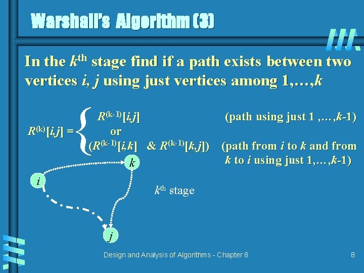
Warshall’s Algorithm (3) In the kth stage find if a path exists between two vertices i, j using just vertices among 1, …, k { R(k)[i, j] = R(k-1)[i, j] (path using just 1 , …, k-1) or (R(k-1)[i, k] & R(k-1)[k, j]) (path from i to k and from k to i using just 1, …, k-1) k i kth stage j Design and Analysis of Algorithms - Chapter 8 8

Warshall’s Algorithm (4) Algorithm Warshall(A[1. . n, 1. . n]) R(0) A for k 1 to n do for i 1 to n do for j 1 to n do R(k)[i, j] R(k-1)[i, j] or R(k-1)[i, k] and R(k-1)[k, j] return R(k) Space and Time efficiency Design and Analysis of Algorithms - Chapter 8 9

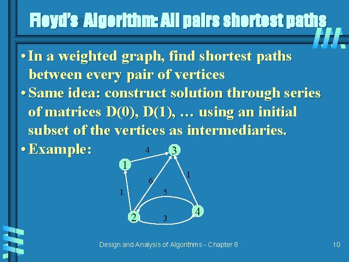
Floyd’s Algorithm: All pairs shortest paths • In a weighted graph, find shortest paths between every pair of vertices • Same idea: construct solution through series of matrices D(0), D(1), … using an initial subset of the vertices as intermediaries. 4 • Example: 3 1 1 6 1 5 2 3 4 Design and Analysis of Algorithms - Chapter 8 10

Floyd’s Algorithm (2) Algorithm Floyd(W[1. . n, 1. . n]) D W for k 1 to n do for i 1 to n do for j 1 to n do D[i, j] min(D[i, j], D[i, k]+D[k, j]) return D • Space and Time efficiency • When does it not work? • Principle of optimality Design and Analysis of Algorithms - Chapter 8 11

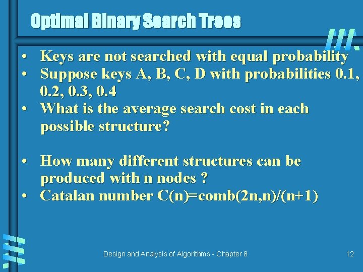
Optimal Binary Search Trees • Keys are not searched with equal probability • Suppose keys A, B, C, D with probabilities 0. 1, 0. 2, 0. 3, 0. 4 • What is the average search cost in each possible structure? • How many different structures can be produced with n nodes ? • Catalan number C(n)=comb(2 n, n)/(n+1) Design and Analysis of Algorithms - Chapter 8 12

Optimal Binary Search Trees (2) • C[i, j] denotes the smallest average search cost in a tree including items i through j • Based on the principle of optimality, the optimal search tree is constructed by using the recurrence C[i, j] = min{C[i, k-1]+C[k+1, j]} + Σps for 1≤i ≤ j ≤ n and i ≤ k ≤ j C[i, i] = pi Design and Analysis of Algorithms - Chapter 8 13

Optimal Binary Search Trees (3) Algorithm Optimal. BST(P[1. . n]) for i 1 to n do C[i, i-1] 0; C[i, i] P[i], R[i, i] I C[n+1, n] 0 for d 1 to n-1 do for i 1 to n-d do j i+d; minval ∞ for k i to j do if C[i, k-1]+C[k+1, j]<minval C[I, k-1]+C[k+1, j]; kmin k R[i, j] kmin; sum P[i]; for s i+1 to j do sum+P[s] C[i, j] minval+sum 14 return C[1, n], Design R and Analysis of Algorithms - Chapter 8

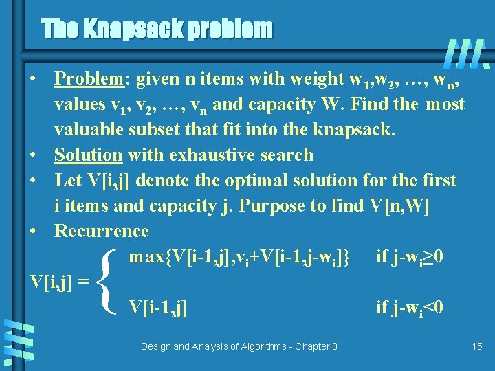
The Knapsack problem • Problem: given n items with weight w 1, w 2, …, wn, values v 1, v 2, …, vn and capacity W. Find the most valuable subset that fit into the knapsack. • Solution with exhaustive search • Let V[i, j] denote the optimal solution for the first i items and capacity j. Purpose to find V[n, W] • Recurrence max{V[i-1, j], vi+V[i-1, j-wi]} if j-wi≥ 0 V[i, j] = V[i-1, j] if j-wi<0 { Design and Analysis of Algorithms - Chapter 8 15

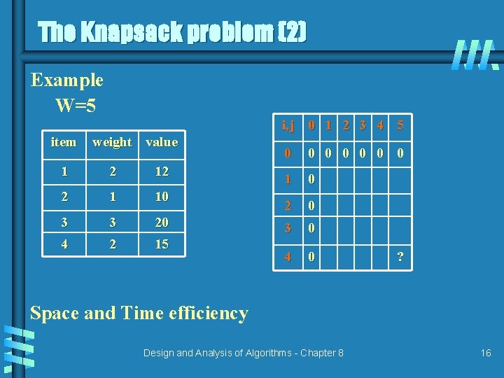
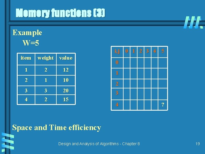
The Knapsack problem (2) Example W=5 i, j 0 1 2 3 4 5 item weight value 1 2 12 2 1 10 3 3 20 4 2 15 0 0 0 0 1 0 2 0 3 0 4 0 ? Space and Time efficiency Design and Analysis of Algorithms - Chapter 8 16

Memory functions [1] A disadvantage of the dynamic programming approach is that is solves subproblems not finally needed. An alternative technique is to combine a topdown and a bottom-up approach (recursion plus a table for temporary results) Design and Analysis of Algorithms - Chapter 8 17

Memory functions [2] Algorithm MFKnapsack(i, j) if V[i, j]<0 if j<Weights[i] value MFKnapack[i-1, j] else value max{MFKnapsack(i-1, j), Values[i]+MFKnapsack[i-1, j-Weights[i]]} V[i, j] value return V[i, j] Design and Analysis of Algorithms - Chapter 8 18

Memory functions (3) Example W=5 i, j 0 1 2 3 4 5 item weight value 1 2 12 2 1 10 3 3 20 4 2 15 0 1 2 3 4 ? Space and Time efficiency Design and Analysis of Algorithms - Chapter 8 19