Detecting Sparse Connectivity MS Lesions Cortical Thickness and

Detecting Sparse Connectivity: MS Lesions, Cortical Thickness, and the ‘Bubbles’ Task in an f. MRI Experiment Keith Worsley, Nicholas Chamandy, Mc. Gill Jonathan Taylor, Stanford and Université de Montréal Robert Adler, Technion Philippe Schyns, Fraser Smith, Glasgow Frédéric Gosselin, Université de Montréal Arnaud Charil, Alan Evans, Montreal Neurological Institute

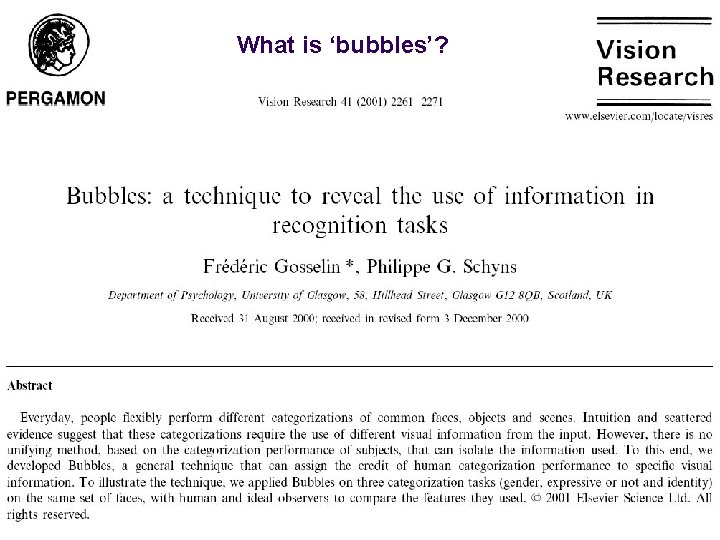
What is ‘bubbles’?

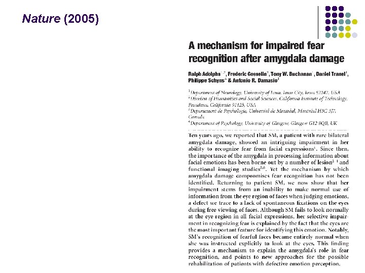
Nature (2005)

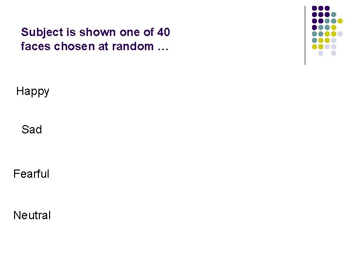
Subject is shown one of 40 faces chosen at random … Happy Sad Fearful Neutral

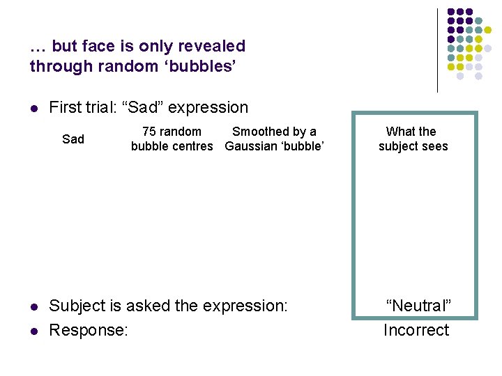
… but face is only revealed through random ‘bubbles’ l First trial: “Sad” expression Sad l l 75 random Smoothed by a bubble centres Gaussian ‘bubble’ Subject is asked the expression: Response: What the subject sees “Neutral” Incorrect

Your turn … l Trial 2 Subject response: “Fearful” CORRECT

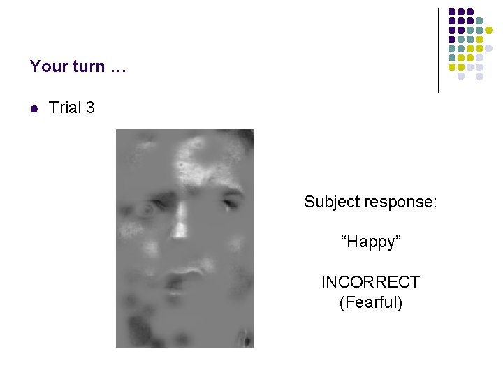
Your turn … l Trial 3 Subject response: “Happy” INCORRECT (Fearful)

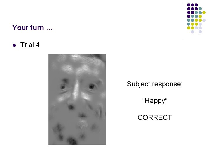
Your turn … l Trial 4 Subject response: “Happy” CORRECT

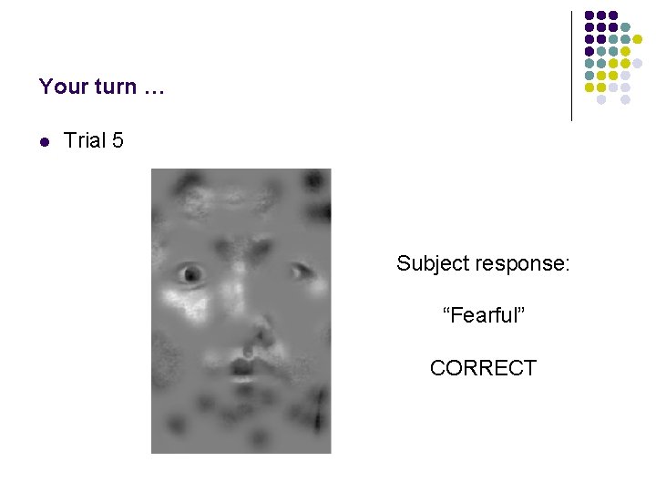
Your turn … l Trial 5 Subject response: “Fearful” CORRECT

Your turn … l Trial 6 Subject response: “Sad” CORRECT

Your turn … l Trial 7 Subject response: “Happy” CORRECT

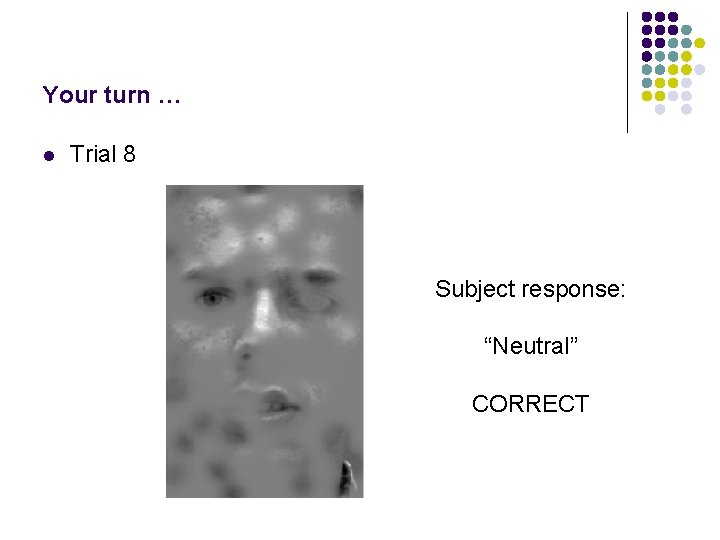
Your turn … l Trial 8 Subject response: “Neutral” CORRECT

Your turn … l Trial 9 Subject response: “Happy” CORRECT

Your turn … l Trial 3000 Subject response: “Happy” INCORRECT (Fearful)

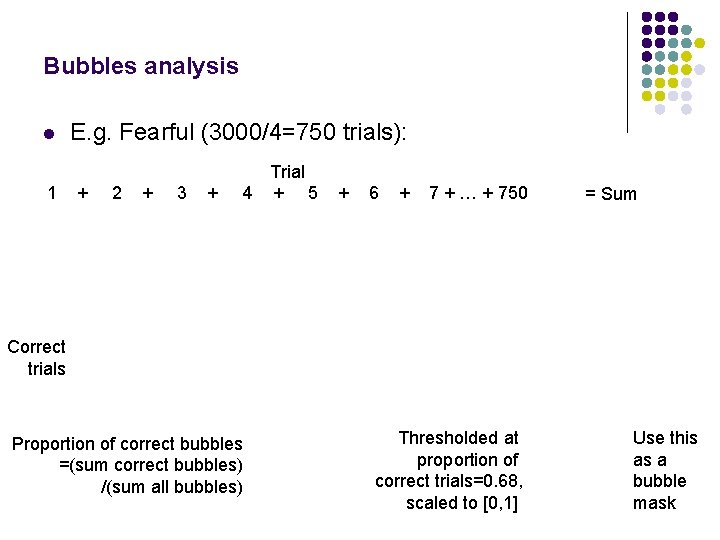
Bubbles analysis l 1 E. g. Fearful (3000/4=750 trials): + 2 + 3 + Trial 4 + 5 + 6 + 7 + … + 750 = Sum Correct trials Proportion of correct bubbles =(sum correct bubbles) /(sum all bubbles) Thresholded at proportion of correct trials=0. 68, scaled to [0, 1] Use this as a bubble mask

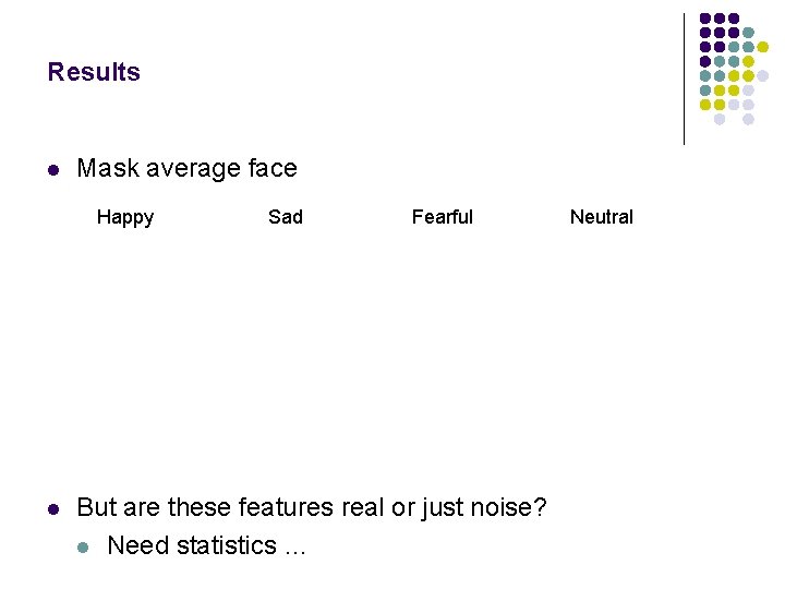
Results l Mask average face Happy l Sad Fearful But are these features real or just noise? l Need statistics … Neutral

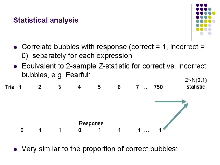
Statistical analysis Correlate bubbles with response (correct = 1, incorrect = 0), separately for each expression Equivalent to 2 -sample Z-statistic for correct vs. incorrect bubbles, e. g. Fearful: l l Trial 1 2 0 l 1 3 4 5 1 Response 0 1 6 1 7 … 1 … 750 1 Very similar to the proportion of correct bubbles: Z~N(0, 1) statistic

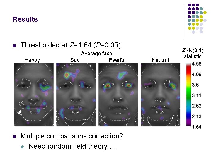
Results l Thresholded at Z=1. 64 (P=0. 05) Happy l Average face Sad Fearful Multiple comparisons correction? l Need random field theory … Neutral Z~N(0, 1) statistic

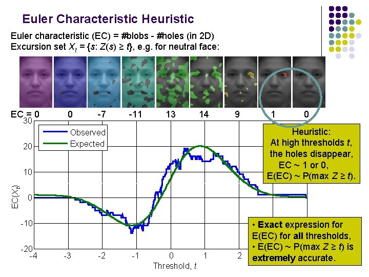
Euler Characteristic Heuristic Euler characteristic (EC) = #blobs - #holes (in 2 D) Excursion set Xt = {s: Z(s) ≥ t}, e. g. for neutral face: EC = 0 30 20 0 -7 -11 13 14 9 0 Heuristic: At high thresholds t, the holes disappear, EC ~ 1 or 0, E(EC) ~ P(max Z ≥ t). Observed Expected 10 EC(Xt) 1 0 -10 -20 -4 -3 -2 -1 0 1 Threshold, t 2 • Exact expression for E(EC) for all thresholds, • E(EC) ~ P(max Z ≥ t) is 3 4 extremely accurate.

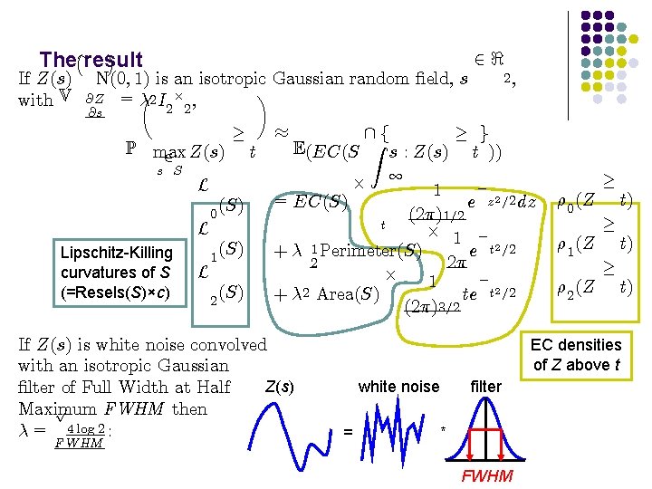
¡ ¢ The» result If Z(s) with V N(0; 1) is an isotropic Gaussian random ¯eld, s µ ¶ @Z = ¸ 2 I £ , @s 2, 2 2 P max 2 Z(s) ¸ t ¼ E(EC(S s S L Lipschitz-Killing curvatures of S (=Resels(S)×c) (S) 0 L (S) 1 L (S) 2 f Z £ ¸ g s : Z(s) t )) 1 ¡ 1 = EC(S) e z 2 =2 dz (2¼)1=2 t £ 1 ¡ + ¸ 1 Perimeter(S) e t 2 =2 2 2¼ £ ¡ 1 2 + ¸ Area(S) te t 2 =2 (2¼)3=2 If Z(s) is white noise convolved with an isotropic Gaussian Z(s) ¯lter of Full Width at Half p Maximum FWHM then ¸ = 4 log 2 : FWHM 2< ½ 0 (Z ½ 1 (Z ½ 2 (Z ¸ t) EC densities of Z above t white noise = filter * FWHM

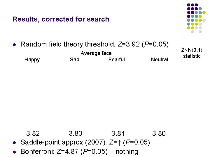
Results, corrected for search l Random field theory threshold: Z=3. 92 (P=0. 05) Happy l l Average face Sad Fearful Neutral 3. 82 3. 80 3. 81 3. 80 Saddle-point approx (2007): Z=↑ (P=0. 05) Bonferroni: Z=4. 87 (P=0. 05) – nothing Z~N(0, 1) statistic

The» result ¡ ¢ If Z(s) N(0; 1) is an isotropic Gaussian random ¯eld, s µ @Z , ¶ with ¸ 2 I 2£ 2 = V @s P max 2 Z(s) ¸ t ¼ E(EC(S s S L Lipschitz-Killing curvatures of S (=Resels(S)×c) (S) 0 L (S) 1 L (S) 2 £ 2, ¸ g s : Z(s) t )) 1 ¡ 1 = EC(S) e z 2 =2 dz (2¼)1=2 t £ 1 ¡ + ¸ 1 Perimeter(S) e t 2 =2 2 2¼ £ ¡ 1 2 + ¸ Area(S) te t 2 =2 (2¼)3=2 If Z(s) is white noise convolved with an isotropic Gaussian Z(s) ¯lter of Full Width at Half p Maximum FWHM then ¸ = 4 log 2 : FWHM f Z 2< ½ 0 (Z ½ 1 (Z ½ 2 (Z ¸ t) EC densities of Z above t white noise = filter * FWHM

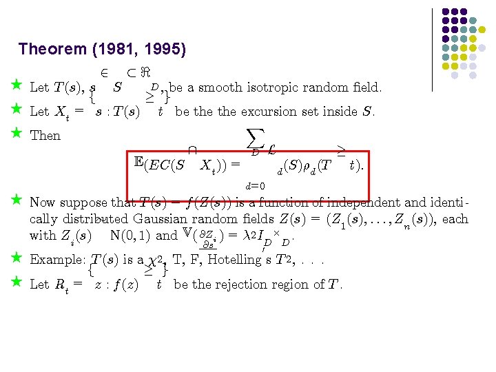
Theorem (1981, 1995) 2 ½< F Let T (s), s S D , be a smooth isotropic random ¯eld. ¸ g f F Let X = s : T (s) t be the excursion set inside S. t X F Then ¸ D L E(EC(S X )) = (S)½d (T t): d t d=0 F Now suppose that T (s) = f (Z(s)) is a function of independent and identi» cally distributed Gaussian random ¯elds Z(s) = (Z 1 (s); : : : ; Zn (s)), each with Zi (s) N(0; 1) and V( @Zi ) = ¸ 2 ID£D. @s 0 F Example: T (s) is a 2 , T, F, Hotelling s T 2 , . . . ¸ g f F Let R = z : f (z) t be the rejection region of T. t

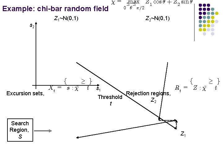
Example: chi-bar random field s 2 Excursion sets, Search Region, S ¹= Z 1~N(0, 1) Z 1 ·max · 0 µ ¼=2 cos µ + Z 2 sin µ Z 2~N(0, 1) ¸ g f Xt = s : ¹ t s 1 Threshold t Rejection regions, Z 2 ¸ g f Rt = Z : ¹ t Z 1

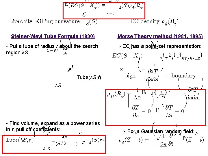
E(EC(S Lipschitz-Killing curvature L d D Xt )) = d (S)½d (Rt ) d=0 (S) Steiner-Weyl Tube Formula (1930) µ ¶ • Put a tube of radius r about @Z the search = ¸ Sd region λS @s r Tube(λS, r) λS • Find volume, expand as a power series X in r, pull off coefficients: j j L D ¼d ¡ (S)r d Tube(¸S; r) = d D ¡(d=2 + 1) d= 0 L EC density ½d (Rt ) Morse Theory. X method (1981, 1995) • EC has a point-set representation: EC(S £ Xµt ) = s ¡ @2 T µ 0 sign @s@s 1¶f. T ¸tg 1 f@T =@s=0 g µ ¶ + boundary ¡ @2 T 1 ¯ E ¶ 0 1 f. T ¸µtg det ¶ ½D (Rt ) = ¯ ¸D @s@s ¯ ¯ @T @T =0 P =0 @s @s µ ¶ ¡ • For¸a Gaussian p random field: ¸ ½d (Z t) = 1 @ 2¼ @t d P(Z t)

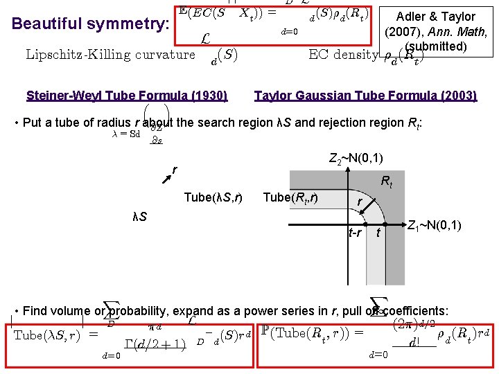
E(EC(S Beautiful symmetry: Lipschitz-Killing curvature L d D Xt )) = L d (S)½d (Rt ) Adler & Taylor (2007), Ann. Math, (submitted) d=0 (S) Steiner-Weyl Tube Formula (1930) µ ¶ EC density ½d (Rt ) Taylor Gaussian Tube Formula (2003) • Put a tube of radius r about @Z the search region λS and rejection region Rt: ¸ = Sd @s Z 2~N(0, 1) r Rt Tube(λS, r) Tube(Rt, r) r λS t-r t X X d= 0 d=0 Z 1~N(0, 1) • Find volume or probability, expand as a power series in r, pull off 1 coefficients: j j L D (2¼)d=2 ¼d P ¡ = ; r)) ½d (Rt )rd (Tube(R = d (S)r Tube(¸S; r) t d D d! ¡(d=2 + 1)

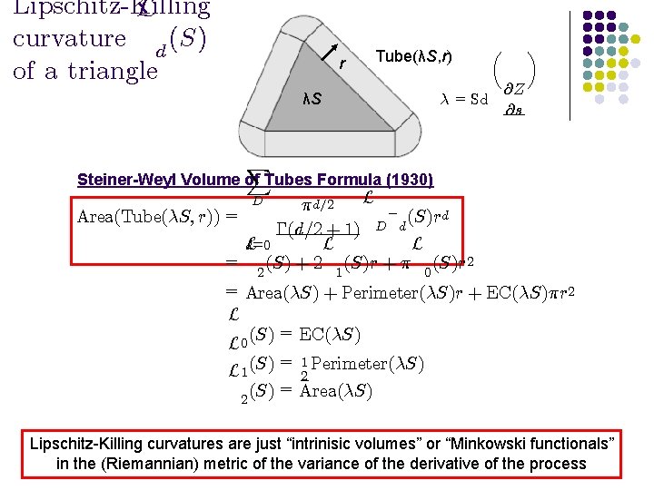
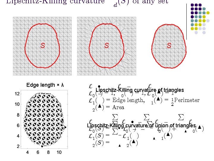
Lipschitz-Killing L curvature d (S) of a triangle r Tube(λS, r) λS ¸ = Sd µ @Z @s ¶ X Steiner-Weyl Volume of Tubes Formula (1930) L ¼ d=2 ¡ (S)r d Area(Tube(¸S; r)) = ¡(d=2 + 1) D d L L L d=0 = (S) + 2 (S)r + ¼ (S)r 2 2 1 0 = Area(¸S) + Perimeter(¸S)r + EC(¸S)¼r 2 L (S) = EC(¸S) L 0 =1 L 1 (S) 2 Perimeter(¸S) (S) = Area(¸S) 2 D Lipschitz-Killing curvatures are just “intrinisic volumes” or “Minkowski functionals” in the (Riemannian) metric of the variance of the derivative of the process

Lipschitz-Killing curvature S Edge length × λ S d (S) of any set S L ² L ¡ L Lipschitz-Killing curvature of triangles L 0 (¡) = 1, 0 ( ) = 1, L 0 (N) = 1 L 1 ( ) = Edge length, 1 (N) = 12 Perimeter (N) = Area 2 P P L ² ¡ PL ¡ L L Lipschitz-Killing curvature of union of triangles L 0 (S) = P² L 0 ( ¡) ¡ ¡ L 0 ( ) + N 0 (N) L 1 (S) = ¡ L 1 ( ) N 1 (S) = N 2 (N) 2

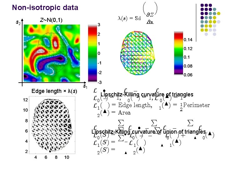
Non-isotropic data s 2 ¸(s) = Sd Z~N(0, 1) Edge length × λ(s) s 1 µ @Z @s ¶ L ² L ¡ L Lipschitz-Killing curvature of triangles L 0 (¡) = 1, 0 ( ) = 1, L 0 (N) = 1 L 1 ( ) = Edge length, 1 (N) = 12 Perimeter (N) = Area 2 P P L ² ¡ PL ¡ L L Lipschitz-Killing curvature of union of triangles L 0 (S) = P² L 0 ( ¡) ¡ ¡ L 0 ( ) + N 0 (N) L 1 (S) = ¡ L 1 ( ) N 1 (S) = N 2 (N) 2

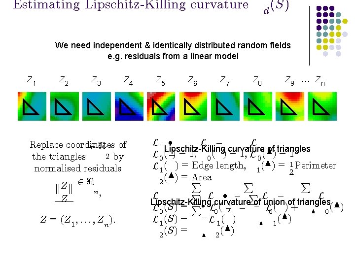
Estimating Lipschitz-Killing curvature d (S) We need independent & identically distributed random fields e. g. residuals from a linear model Z 1 Z 2 Z 3 Z 4 Replace coordinates 2 < of 2 by the triangles normalised residuals 2< Z jj jj n; Z Z = (Z 1 ; : : : ; Zn ): Z 5 Z 6 Z 7 Z 8 Z 9 … Zn L ² L ¡ L Lipschitz-Killing curvature of triangles L 0 (¡) = 1, 0 ( ) = 1, L 0 (N) = 1 L 1 ( ) = Edge length, 1 (N) = 12 Perimeter Area (N) = P P P 2 P L ² ¡ PL ¡ L L Lipschitz-Killing curvature of union of triangles L 0 (S) = P² L 0 ( ¡) ¡ ¡ L 0 ( ) + N 0 (N) L 1 (S) = ¡ L 1 ( ) N 1 (S) = N 2 (N) 2

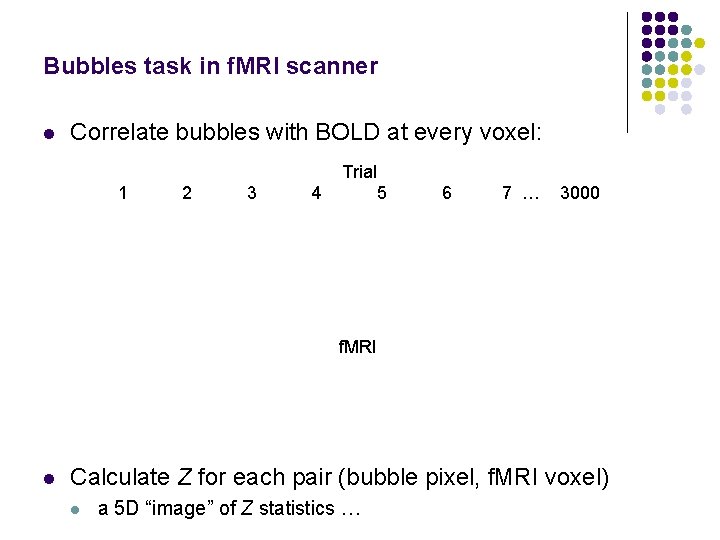
Bubbles task in f. MRI scanner l Correlate bubbles with BOLD at every voxel: Trial 1 2 3 4 5 6 7 … 3000 f. MRI l Calculate Z for each pair (bubble pixel, f. MRI voxel) l a 5 D “image” of Z statistics …

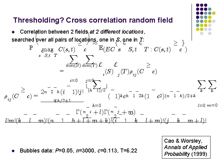
Thresholding? Cross correlation random field µ ¶ Correlation between 2 fields at 2 different locations, searched over all pairs of locations, one in S, one in T: l P 2 max 2 s S; t T ¸ C(s; t) c X X = ½ij (C c) = ¡ ¡ 2 n 2 h (i ¸ g 2 f 2 E(EC s S; t T : C(s; t) c ) ¸ L (S) j (T )½ij (C c) i dim(S) dim(T ) L i=0 ¸ ¼ ¡ ¼ h=2+1 1)!j! j =0 X b ¡ c (h 1)=2 ¡ ¡ ¡ ( 1)k ch 1 2 k (1 c 2 )(n 1 h)=2+k ¡ ¡ k=0 ¡( n i + l)¡( n j¡+ 2 2 ¡ ¡ l!m!(k l m)!(n 1 h + l + m + k)!(i l XX k l=0 m) ¡ ¡ 1 k l + m)!(j k m + l)! Bubbles data: P=0. 05, n=3000, c=0. 113, T=6. 22 k Cao & Worsley, Annals of Applied Probability (1999)

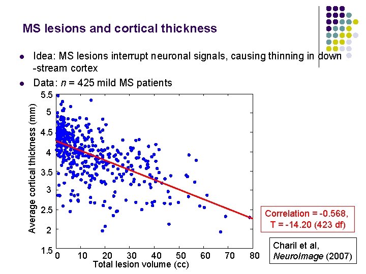
MS lesions and cortical thickness l Idea: MS lesions interrupt neuronal signals, causing thinning in down -stream cortex Data: n = 425 mild MS patients 5. 5 Average cortical thickness (mm) l 5 4 3. 5 3 2. 5 Correlation = -0. 568, T = -14. 20 (423 df) 2 1. 5 0 10 20 30 40 50 Total lesion volume (cc) 60 70 80 Charil et al, Neuro. Image (2007)

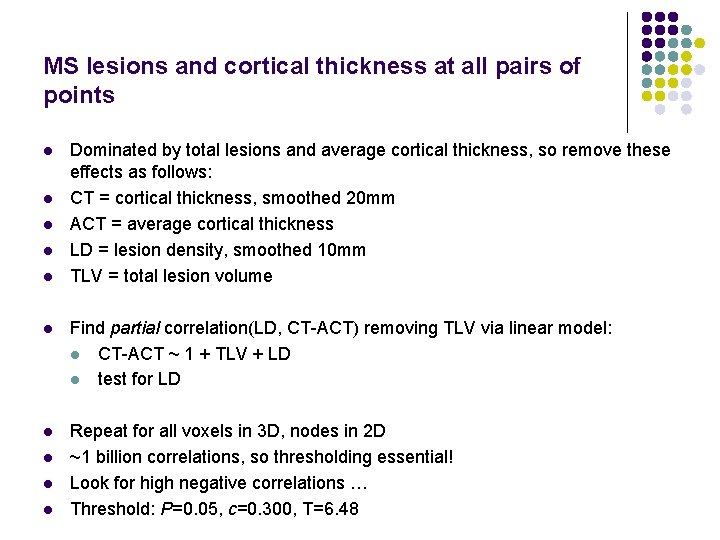
MS lesions and cortical thickness at all pairs of points l l l Dominated by total lesions and average cortical thickness, so remove these effects as follows: CT = cortical thickness, smoothed 20 mm ACT = average cortical thickness LD = lesion density, smoothed 10 mm TLV = total lesion volume l Find partial correlation(LD, CT-ACT) removing TLV via linear model: l CT-ACT ~ 1 + TLV + LD l test for LD l Repeat for all voxels in 3 D, nodes in 2 D ~1 billion correlations, so thresholding essential! Look for high negative correlations … Threshold: P=0. 05, c=0. 300, T=6. 48 l l l

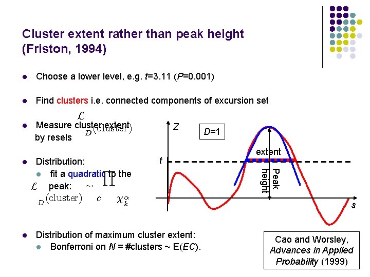
Cluster extent rather than peak height (Friston, 1994) l Choose a lower level, e. g. t=3. 11 (P=0. 001) l Find clusters i. e. connected components of excursion set l l L Measure cluster extent (cluster) D by resels D l (cluster) c t ® k Distribution of maximum cluster extent: l Bonferroni on N = #clusters ~ E(EC). D=1 extent Peak height Distribution: Y l fit a quadratic to the L peak: » Z s Cao and Worsley, Advances in Applied Probability (1999)