Details Homework 4 due Today Extra Credit Homework

Details • • Homework #4 due Today Extra Credit Homework due Thurs 3/18 Reading, Chapter 7 pages 210 -216 & 220 -224 Final Exam, Tuesday March 23, 8: 00 -10: 00 am – Bring: • • Scantron F-288 ERI-L #2 Pencil Calculator 8 ½ x 11 page of notes • Pick up a registration code for 10 C

T-test and Confidence intervals for difference between two means Small Samples • T statistic and T Test – Standard error – Assumptions – Examples • Confidence intervals for small samples

If one or both of the samples is smaller than 20 • Assume that the population distributions are approximately normal • Also, assume that population variances are equal

Hypothesis Tests for Two Sample Means • Interval Level Dependent Variable • Nominal Level Independent Variable

Small Sample test for two means • • • Assumptions Independent random samples Interval level dependent variable Nominal level independent variable Size of either sample is < 20 • Population variances are equal • Population distributions are normal

T test for the difference between two means

Exact T test if • Variances are assumed equal Estimate a common standard deviation

Estimated Standard Error I hope SPSS calculates this for me !

Sampling distribution of the difference between two means Small Samples • Mean • Standard error • Shape, T Distribution • (Assume equal variances and normal population distributions)

Example, Type of transportation and travel time to work 1990 US Census Motorcycles and Bicycles

Steps • State the assumptions • State the null hypothesis and the research hypothesis and select alpha • Select the appropriate statistical test • Compute the test statistic • Make a decision about the hypothesis and state a conclusion

Hypotheses & Significance Level • Null Hypothesis: Mean commute times by motorcycle are not different from mean commute times by bicycle. • Alternative Hypothesis: Mean commute times by motorcycle are longer than mean commute times by bicycle. • Alpha =. 01

Travel time to work for two means of transportation

Difference between means • Motorcycle – Bicycle

Estimate the standard error • Variances are assumed equal

Estimate the standard error

Estimate the standard error

Estimate the standard error

Compute the test statistic

Compute the test statistic

Sampling distribution of the difference between means

t distribution 0

Degrees of freedom • Population variances assumed equal or both N 1 and N 2 are larger than 20 • Population variances unequal and one or both of N 1 and N 2 is less than 20

Degrees of freedom • Population variances assumed equal or both N 1 and N 2 are larger than 20

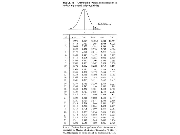
Decision about the null hypothesis • The hypothesis is directional, so use a onetailed test • Significance level, alpha =. 01 • Degrees of freedom, df = 38

Alpha =. 01 df=38 Critical value of t is 2. 326

Decision about the null hypothesis • The critical value of t is 2. 326 • The obtained t = 1. 56 Critical value of t= 2. 326 Obtained value of t = 1. 56

P value for obtained t Obtained value of t = 1. 56

One-tailed P value is Between. 1 and. 05 df=38 Obtained value of t = 1. 56

Decision about Hypotheses & Conclusion • Null Hypothesis: Mean commute times by bicycle are not different from mean commute times by motorcycle. • Alternative Hypothesis: Mean commute times by motorcycle are longer than mean commute times by bicycle. Obtained value of t = 1. 56 • Alpha =. 01 P value >. 05 Critical value of t= 2. 326

Conclusion • For a sample of N=18 people, the mean commute time by motorcycle is 16. 44 minutes • For a sample of N=20 people, the mean commute time by bicycle is 11. 86 minutes • The independent samples t-test for this difference is t=1. 56, with d. f. =38 (p>. 05) therefore we cannot reject the null hypothesis that there is no difference in mean commute times between bicycles and motorcycles.

Small Sample Confidence Interval for difference between means

95% CI df=38

T Table df=38 t=2. 021

95% Confidence Interval t=2. 021

95% Confidence Interval From – 1. 36 to 10. 52 t=2. 021

95% Confidence Interval for the difference in commute times between motorcycle and bicycle From – 1. 36 to 10. 52 We can be 95% confident that mean commute times by motorcycle are between 1. 36 minutes shorter and 10. 52 minutes longer than mean commute times by bicycle Notice that the interval includes 0 as a possibility

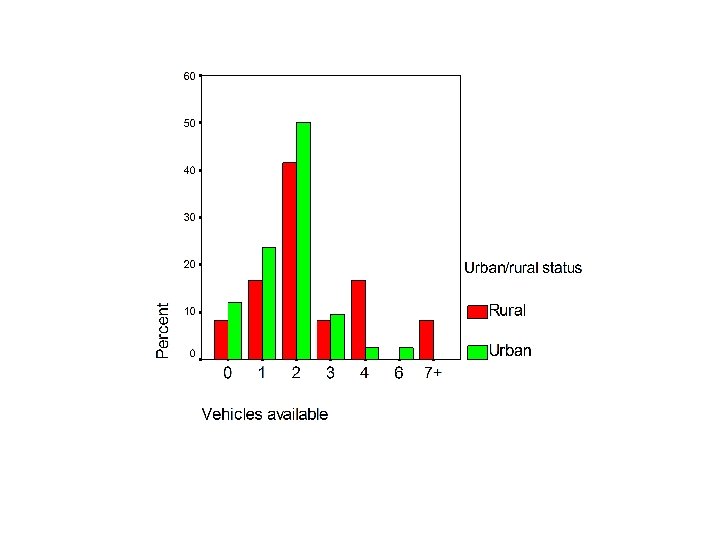
Another Example • The number of vehicles • In urban and rural areas • Data from 1990 US Census • Use Alpha =. 05 What are the variables here?

Hypotheses • Null Hypothesis: The mean number of vehicles available is not different in rural and urban areas • Alternative Hypothesis: The mean number of vehicles available is different in rural and urban areas

Number of Vehicles

Let SPSS do some of the work !

Let SPSS do some of the work !

Two-tailed P value is Between. 05 and. 1 df=52 A two tailed test Double the probabilities Obtained value of t = +1. 73

Alpha =. 05 ½ of. 05 =. 025 Critical values of t= +/- 1. 96 df=52

Let SPSS do some of the work !

Decision about the null hypothesis Alpha =. 05 Two-tailed P value is Between. 05 and. 1 Critical value of t= -1. 96 Critical value of t= +1. 96 Obtained value of t = +1. 73

Decision about the null hypothesis • Null Hypothesis: The mean number of vehicles available is not different in rural and urban areas Using a. 05 significance level • Alternative mean number Do not. Hypothesis: reject the null. The hypothesis Thereavailable is no significant difference of vehicles is different in rural and between the mean number of vehicles available urban areas in rural and urban areas

95% Confidence Interval for difference between means

95% CI df=52 t=+/- 1. 96

95% Confidence Interval for difference between means t=+/- 1. 96

95% Confidence Interval for difference between means t=+/- 1. 96

95% Confidence Interval for difference between means

95% Confidence Interval for difference between mean number of vehicles in rural and urban areas • We can be 95% confident that the mean number of vehicles in rural areas is ……

95% CI df=38

Estimate the common standard deviation • Variances are assumed equal

Estimate the common standard deviation • Variances are assumed equal

Estimate the common standard deviation • Variances are assumed equal

Hypotheses & Significance Level • Null Hypothesis: Mean commute times by motorcycle are not different from mean commute times by bicycle. • Alternative Hypothesis: Mean commute times by motorcycle are longer than mean commute times by bicycle. • Alpha =. 01

Difference between means • Motorcycle – Bicycle

SPSS output – Independent samples t test