Data WarehousingMining Comp 150 DW Chapter 6 Mining

Data Warehousing/Mining Comp 150 DW Chapter 6: Mining Association Rules in Large Databases Instructor: Dan Hebert Data Warehousing/Mining 1

Chapter 6: Mining Association Rules in Large Databases v Association rule mining v Mining single-dimensional Boolean association rules from transactional databases v DBMiner v Mining multilevel association rules from transactional databases v Mining multidimensional association rules from transactional databases and data warehouse v From association mining to correlation analysis v Constraint-based association mining v Summary Data Warehousing/Mining 2

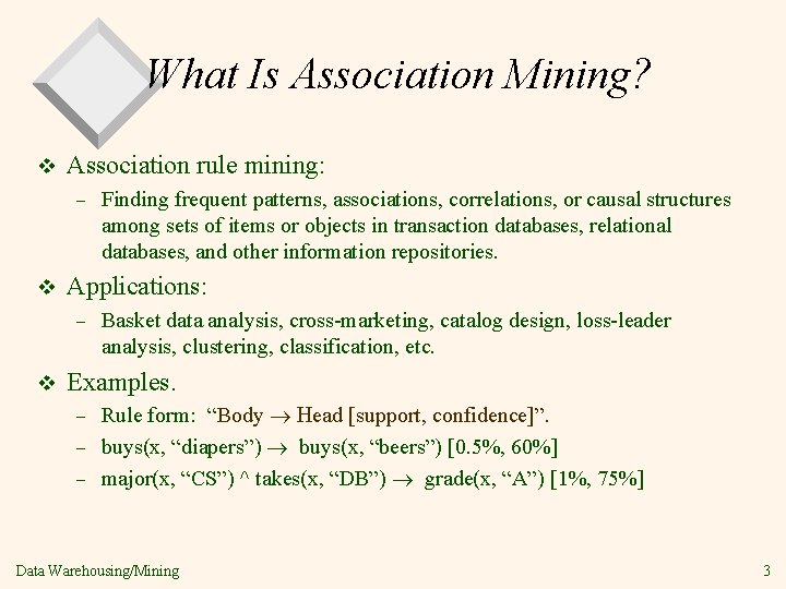
What Is Association Mining? v Association rule mining: – v Applications: – v Finding frequent patterns, associations, correlations, or causal structures among sets of items or objects in transaction databases, relational databases, and other information repositories. Basket data analysis, cross-marketing, catalog design, loss-leader analysis, clustering, classification, etc. Examples. Rule form: “Body ® Head [support, confidence]”. – buys(x, “diapers”) ® buys(x, “beers”) [0. 5%, 60%] – major(x, “CS”) ^ takes(x, “DB”) ® grade(x, “A”) [1%, 75%] – Data Warehousing/Mining 3

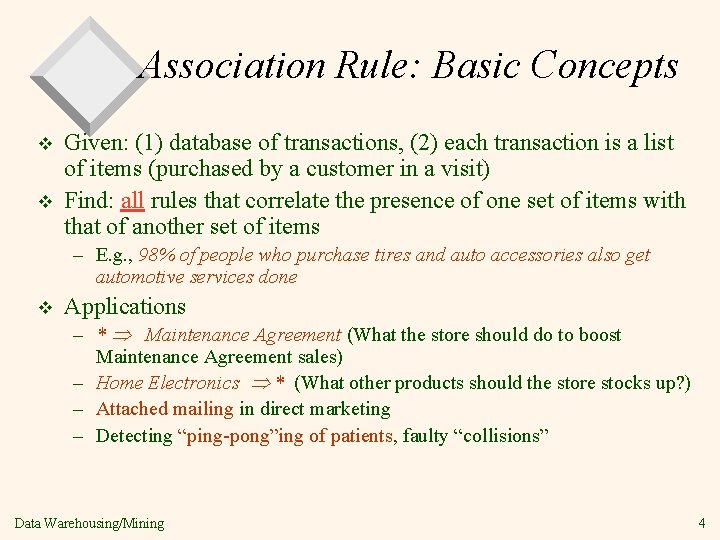
Association Rule: Basic Concepts v v Given: (1) database of transactions, (2) each transaction is a list of items (purchased by a customer in a visit) Find: all rules that correlate the presence of one set of items with that of another set of items – E. g. , 98% of people who purchase tires and auto accessories also get automotive services done v Applications – * Maintenance Agreement (What the store should do to boost Maintenance Agreement sales) – Home Electronics * (What other products should the store stocks up? ) – Attached mailing in direct marketing – Detecting “ping-pong”ing of patients, faulty “collisions” Data Warehousing/Mining 4

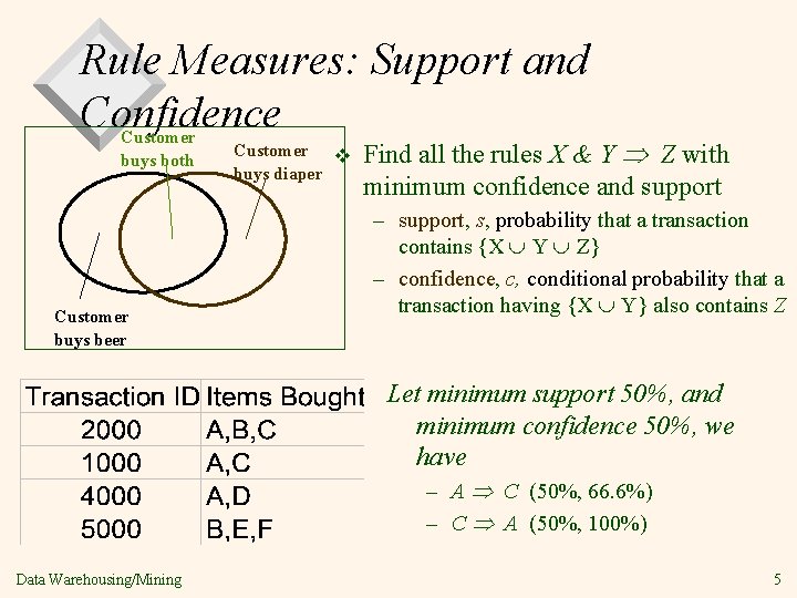
Rule Measures: Support and Confidence Customer buys both Customer buys beer Customer v buys diaper Find all the rules X & Y Z with minimum confidence and support – support, s, probability that a transaction contains {X Y Z} – confidence, c, conditional probability that a transaction having {X Y} also contains Z Let minimum support 50%, and minimum confidence 50%, we have – A C (50%, 66. 6%) – C A (50%, 100%) Data Warehousing/Mining 5

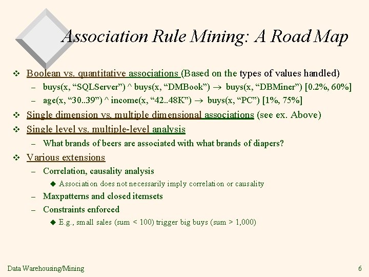
Association Rule Mining: A Road Map v Boolean vs. quantitative associations (Based on the types of values handled) buys(x, “SQLServer”) ^ buys(x, “DMBook”) ® buys(x, “DBMiner”) [0. 2%, 60%] – age(x, “ 30. . 39”) ^ income(x, “ 42. . 48 K”) ® buys(x, “PC”) [1%, 75%] – Single dimension vs. multiple dimensional associations (see ex. Above) v Single level vs. multiple-level analysis v – v What brands of beers are associated with what brands of diapers? Various extensions – Correlation, causality analysis u Association does not necessarily imply correlation or causality Maxpatterns and closed itemsets – Constraints enforced – u E. g. , small sales (sum < 100) trigger big buys (sum > 1, 000) Data Warehousing/Mining 6

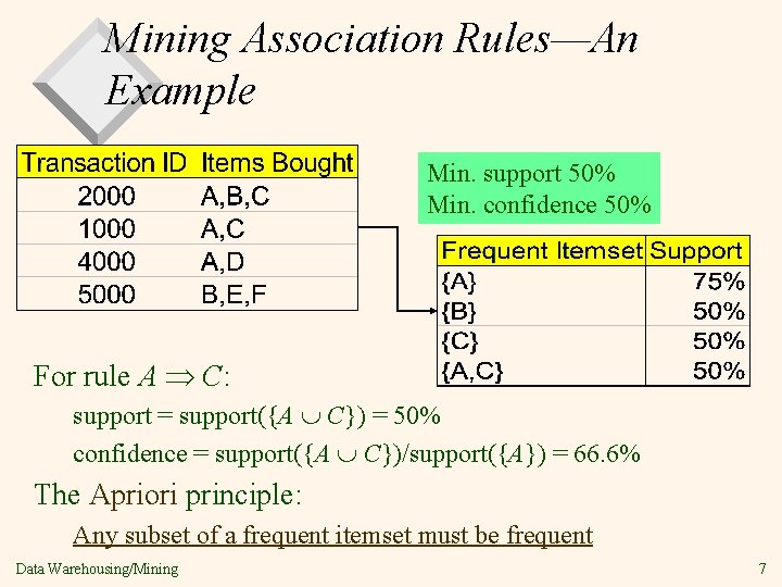
Mining Association Rules—An Example Min. support 50% Min. confidence 50% For rule A C: support = support({A C}) = 50% confidence = support({A C})/support({A}) = 66. 6% The Apriori principle: Any subset of a frequent itemset must be frequent Data Warehousing/Mining 7

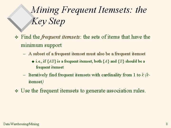
Mining Frequent Itemsets: the Key Step v Find the frequent itemsets: the sets of items that have the minimum support – A subset of a frequent itemset must also be a frequent itemset u i. e. , if {AB} is a frequent itemset, both {A} and {B} should be a frequent itemset – Iteratively find frequent itemsets with cardinality from 1 to k (kitemset) v Use the frequent itemsets to generate association rules. Data Warehousing/Mining 8

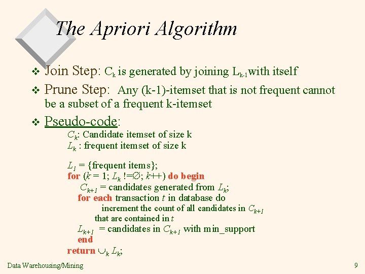
The Apriori Algorithm Join Step: Ck is generated by joining Lk-1 with itself v Prune Step: Any (k-1)-itemset that is not frequent cannot v be a subset of a frequent k-itemset v Pseudo-code: Ck: Candidate itemset of size k Lk : frequent itemset of size k L 1 = {frequent items}; for (k = 1; Lk != ; k++) do begin Ck+1 = candidates generated from Lk; for each transaction t in database do increment the count of all candidates in Ck+1 that are contained in t Lk+1 = candidates in Ck+1 with min_support end return k Lk; Data Warehousing/Mining 9

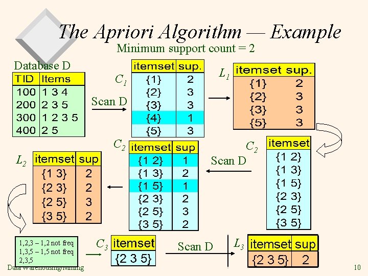
The Apriori Algorithm — Example Minimum support count = 2 Database D L 1 C 1 Scan D C 2 L 2 1, 2, 3 – 1, 2 not freq 1, 3, 5 – 1, 5 not freq 2, 3, 5 Data Warehousing/Mining C 3 C 2 Scan D L 3 itemset sup {2 3 5} 2 10

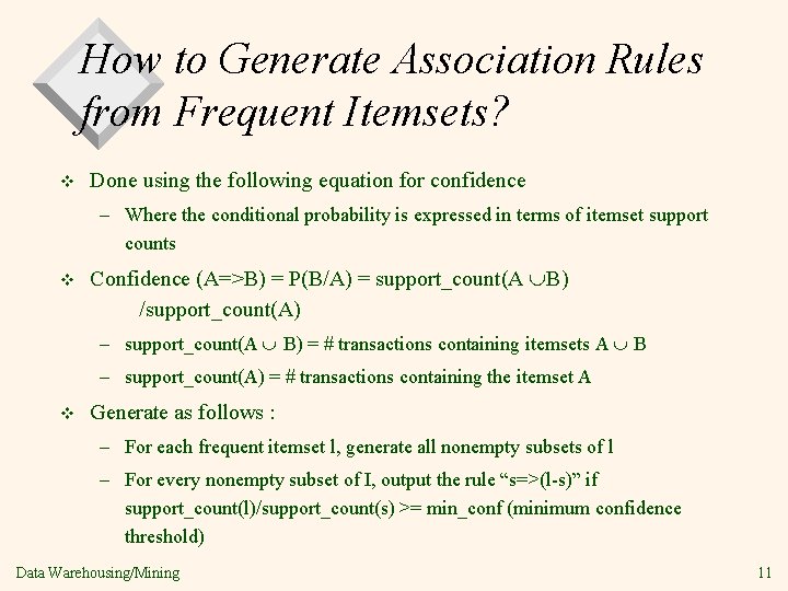
How to Generate Association Rules from Frequent Itemsets? v Done using the following equation for confidence – Where the conditional probability is expressed in terms of itemset support counts v Confidence (A=>B) = P(B/A) = support_count(A B) /support_count(A) – support_count(A B) = # transactions containing itemsets A B – support_count(A) = # transactions containing the itemset A v Generate as follows : – For each frequent itemset l, generate all nonempty subsets of l – For every nonempty subset of I, output the rule “s=>(l-s)” if support_count(l)/support_count(s) >= min_conf (minimum confidence threshold) Data Warehousing/Mining 11

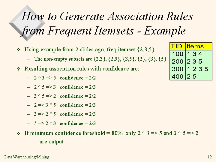
How to Generate Association Rules from Frequent Itemsets - Example v Using example from 2 slides ago, freq itemset {2, 3, 5} – The non-empty subsets are {2, 3}, {2, 5}, {3, 5}, {2}, {3}, {5} v Resulting association rules with confidence are: – 2 ^ 3 => 5 confidence = 2/2 – 2 ^ 5 => 3 confidence = 2/3 – 3 ^ 5 => 2 confidence = 2/2 – 2 => 3 ^ 5 confidence = 2/3 – 3 => 2 ^ 5 confidence = 2/3 – 5 => 2 ^ 3 confidence = 2/3 v If minimum confidence threshold = 80%, only 2 ^ 3 => 5 and 3 ^ 5 => 2 are output Data Warehousing/Mining 12

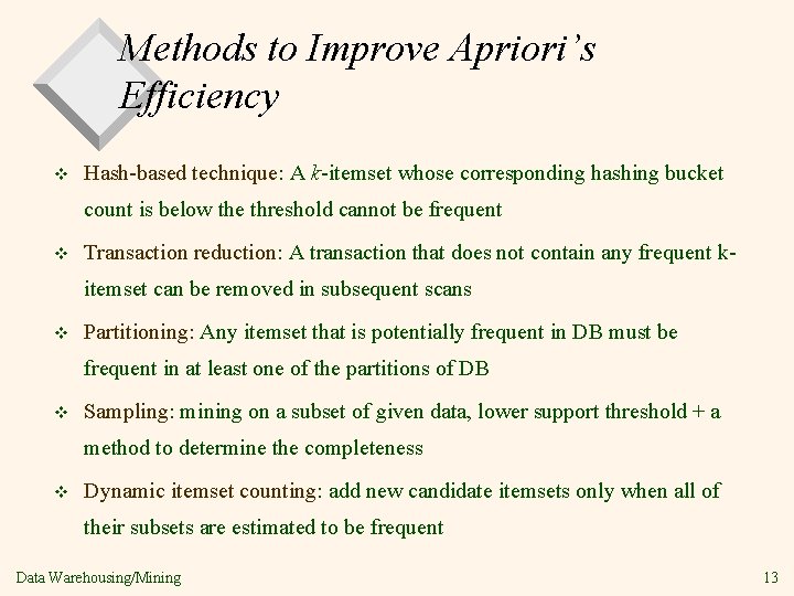
Methods to Improve Apriori’s Efficiency v Hash-based technique: A k-itemset whose corresponding hashing bucket count is below the threshold cannot be frequent v Transaction reduction: A transaction that does not contain any frequent kitemset can be removed in subsequent scans v Partitioning: Any itemset that is potentially frequent in DB must be frequent in at least one of the partitions of DB v Sampling: mining on a subset of given data, lower support threshold + a method to determine the completeness v Dynamic itemset counting: add new candidate itemsets only when all of their subsets are estimated to be frequent Data Warehousing/Mining 13

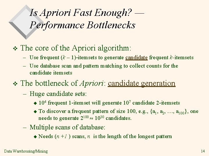
Is Apriori Fast Enough? — Performance Bottlenecks v The core of the Apriori algorithm: – Use frequent (k – 1)-itemsets to generate candidate frequent k-itemsets – Use database scan and pattern matching to collect counts for the candidate itemsets v The bottleneck of Apriori: candidate generation – Huge candidate sets: 104 frequent 1 -itemset will generate 107 candidate 2 -itemsets u To discover a frequent pattern of size 100, e. g. , {a 1, a 2, …, a 100}, one needs to generate 2100 1030 candidates. u – Multiple scans of database: u Needs (n +1 ) scans, n is the length of the longest pattern Data Warehousing/Mining 14

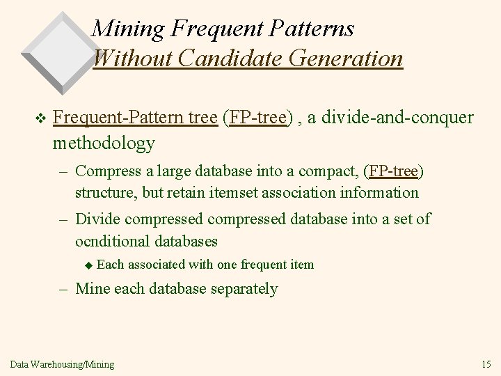
Mining Frequent Patterns Without Candidate Generation v Frequent-Pattern tree (FP-tree) , a divide-and-conquer methodology – Compress a large database into a compact, (FP-tree) structure, but retain itemset association information – Divide compressed database into a set of ocnditional databases u Each associated with one frequent item – Mine each database separately Data Warehousing/Mining 15

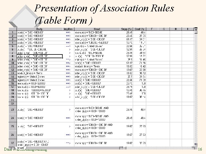
Presentation of Association Rules (Table Form ) Data Warehousing/Mining 16

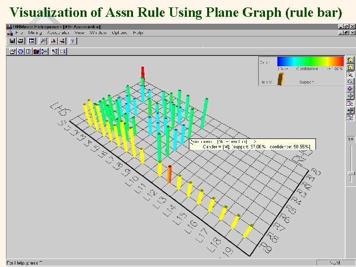
Visualization of Assn Rule Using Plane Graph (rule bar) Data Warehousing/Mining 17

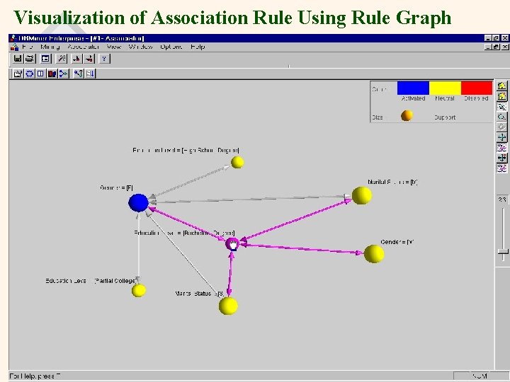
Visualization of Association Rule Using Rule Graph Data Warehousing/Mining 18

DBMiner Examples v Show Examples 1 - 11 Data Warehousing/Mining 19

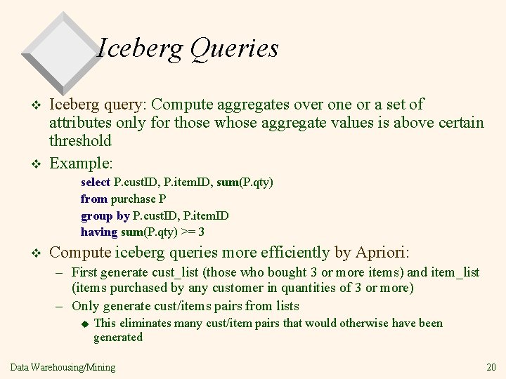
Iceberg Queries v v Iceberg query: Compute aggregates over one or a set of attributes only for those whose aggregate values is above certain threshold Example: select P. cust. ID, P. item. ID, sum(P. qty) from purchase P group by P. cust. ID, P. item. ID having sum(P. qty) >= 3 v Compute iceberg queries more efficiently by Apriori: – First generate cust_list (those who bought 3 or more items) and item_list (items purchased by any customer in quantities of 3 or more) – Only generate cust/items pairs from lists u This eliminates many cust/item pairs that would otherwise have been generated Data Warehousing/Mining 20

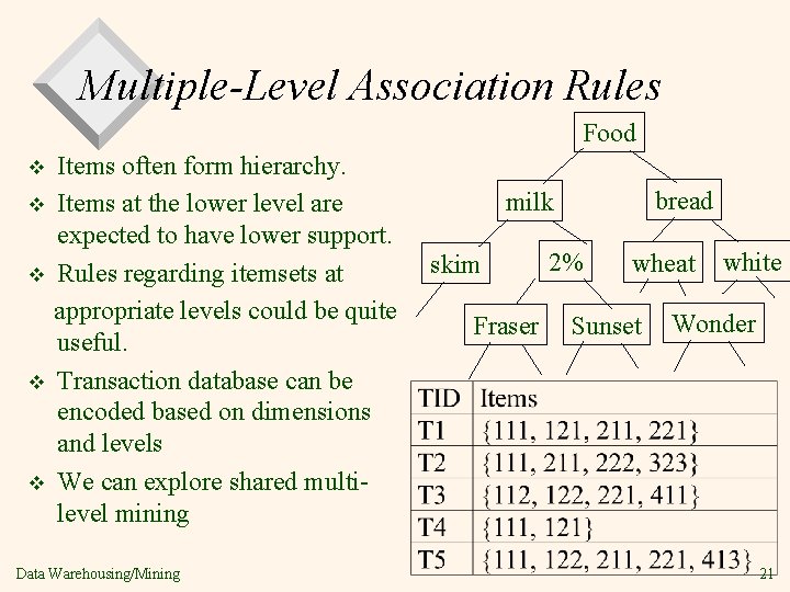
Multiple-Level Association Rules Food v v v Items often form hierarchy. Items at the lower level are expected to have lower support. Rules regarding itemsets at appropriate levels could be quite useful. Transaction database can be encoded based on dimensions and levels We can explore shared multilevel mining Data Warehousing/Mining bread milk skim Fraser 2% wheat Sunset white Wonder 21

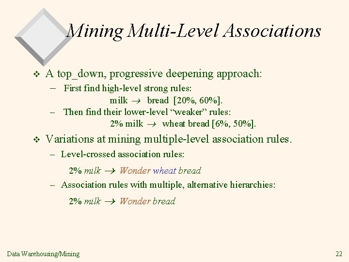
Mining Multi-Level Associations v A top_down, progressive deepening approach: – First find high-level strong rules: milk ® bread [20%, 60%]. – Then find their lower-level “weaker” rules: 2% milk ® wheat bread [6%, 50%]. v Variations at mining multiple-level association rules. – Level-crossed association rules: 2% milk ® Wonder wheat bread – Association rules with multiple, alternative hierarchies: 2% milk ® Wonder bread Data Warehousing/Mining 22

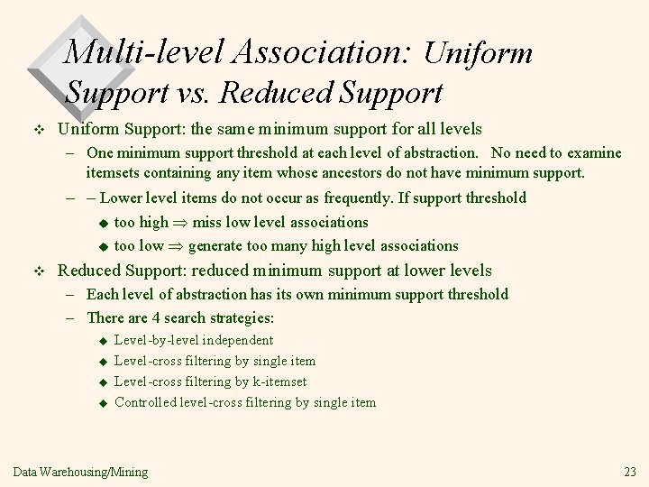
Multi-level Association: Uniform Support vs. Reduced Support v Uniform Support: the same minimum support for all levels – One minimum support threshold at each level of abstraction. No need to examine itemsets containing any item whose ancestors do not have minimum support. – – Lower level items do not occur as frequently. If support threshold u u v too high miss low level associations too low generate too many high level associations Reduced Support: reduced minimum support at lower levels – Each level of abstraction has its own minimum support threshold – There are 4 search strategies: u u Level-by-level independent Level-cross filtering by single item Level-cross filtering by k-itemset Controlled level-cross filtering by single item Data Warehousing/Mining 23

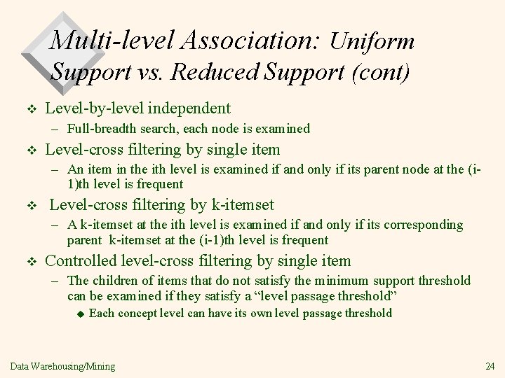
Multi-level Association: Uniform Support vs. Reduced Support (cont) v Level-by-level independent – Full-breadth search, each node is examined v Level-cross filtering by single item – An item in the ith level is examined if and only if its parent node at the (i 1)th level is frequent v Level-cross filtering by k-itemset – A k-itemset at the ith level is examined if and only if its corresponding parent k-itemset at the (i-1)th level is frequent v Controlled level-cross filtering by single item – The children of items that do not satisfy the minimum support threshold can be examined if they satisfy a “level passage threshold” u Each concept level can have its own level passage threshold Data Warehousing/Mining 24

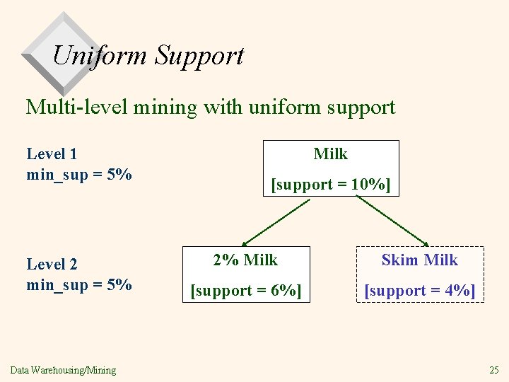
Uniform Support Multi-level mining with uniform support Level 1 min_sup = 5% Level 2 min_sup = 5% Data Warehousing/Mining Milk [support = 10%] 2% Milk Skim Milk [support = 6%] [support = 4%] 25

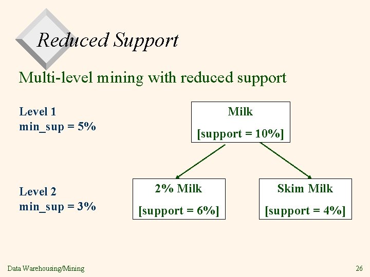
Reduced Support Multi-level mining with reduced support Level 1 min_sup = 5% Level 2 min_sup = 3% Data Warehousing/Mining Milk [support = 10%] 2% Milk Skim Milk [support = 6%] [support = 4%] 26

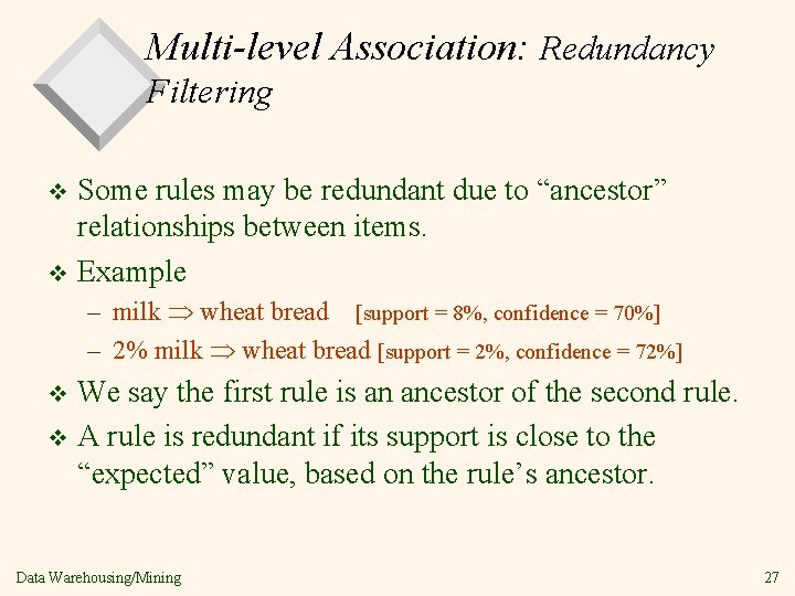
Multi-level Association: Redundancy Filtering Some rules may be redundant due to “ancestor” relationships between items. v Example v – milk wheat bread [support = 8%, confidence = 70%] – 2% milk wheat bread [support = 2%, confidence = 72%] We say the first rule is an ancestor of the second rule. v A rule is redundant if its support is close to the “expected” value, based on the rule’s ancestor. v Data Warehousing/Mining 27

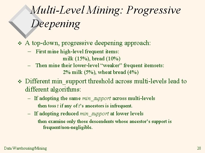
Multi-Level Mining: Progressive Deepening v A top-down, progressive deepening approach: – First mine high-level frequent items: milk (15%), bread (10%) – Then mine their lower-level “weaker” frequent itemsets: 2% milk (5%), wheat bread (4%) v Different min_support threshold across multi-levels lead to different algorithms: – If adopting the same min_support across multi-levels then toss t if any of t’s ancestors is infrequent. – If adopting reduced min_support at lower levels then examine only those descendents whose ancestor’s support is frequent/non-negligible. Data Warehousing/Mining 28

Progressive Refinement of Data Mining Quality v Why progressive refinement? – Mining operator can be expensive or cheap, fine or rough – Trade speed with quality: step-by-step refinement. v Superset coverage property: – Preserve all the positive answers—allow a positive false test but not a false negative test. v Two- or multi-step mining: – First apply rough/cheap operator (superset coverage) – Then apply expensive algorithm on a substantially reduced candidate set Data Warehousing/Mining 29

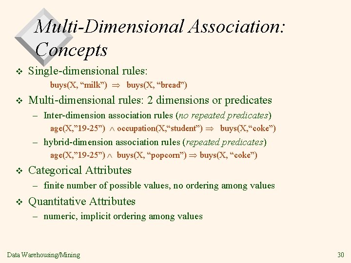
Multi-Dimensional Association: Concepts v Single-dimensional rules: buys(X, “milk”) buys(X, “bread”) v Multi-dimensional rules: 2 dimensions or predicates – Inter-dimension association rules (no repeated predicates) age(X, ” 19 -25”) occupation(X, “student”) buys(X, “coke”) – hybrid-dimension association rules (repeated predicates) age(X, ” 19 -25”) buys(X, “popcorn”) buys(X, “coke”) v Categorical Attributes – finite number of possible values, no ordering among values v Quantitative Attributes – numeric, implicit ordering among values Data Warehousing/Mining 30

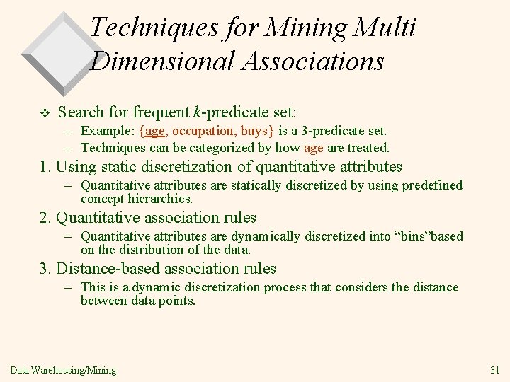
Techniques for Mining Multi Dimensional Associations v Search for frequent k-predicate set: – Example: {age, occupation, buys} is a 3 -predicate set. – Techniques can be categorized by how age are treated. 1. Using static discretization of quantitative attributes – Quantitative attributes are statically discretized by using predefined concept hierarchies. 2. Quantitative association rules – Quantitative attributes are dynamically discretized into “bins”based on the distribution of the data. 3. Distance-based association rules – This is a dynamic discretization process that considers the distance between data points. Data Warehousing/Mining 31

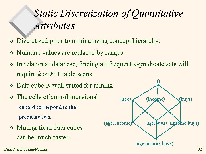
Static Discretization of Quantitative Attributes v Discretized prior to mining using concept hierarchy. v Numeric values are replaced by ranges. v In relational database, finding all frequent k-predicate sets will require k or k+1 table scans. v Data cube is well suited for mining. v The cells of an n-dimensional () (age) (income) (buys) cuboid correspond to the predicate sets. v Mining from data cubes can be much faster. Data Warehousing/Mining (age, income) (age, buys) (income, buys) (age, income, buys) 32

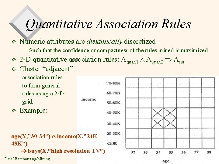
Quantitative Association Rules v Numeric attributes are dynamically discretized – Such that the confidence or compactness of the rules mined is maximized. v v 2 -D quantitative association rules: Aquan 1 Aquan 2 Acat Cluster “adjacent” association rules to form general rules using a 2 -D grid. v Example: age(X, ” 30 -34”) income(X, ” 24 K 48 K”) buys(X, ”high resolution TV”) Data Warehousing/Mining 33

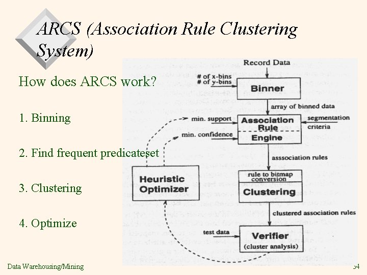
ARCS (Association Rule Clustering System) How does ARCS work? 1. Binning 2. Find frequent predicateset 3. Clustering 4. Optimize Data Warehousing/Mining 34

Limitations of ARCS v Only quantitative attributes on LHS of rules. v Only 2 attributes on LHS. (2 D limitation) v An alternative to ARCS – Non-grid-based – equi-depth binning – clustering based on a measure of partial completeness. – “Mining Quantitative Association Rules in Large Relational Tables” by R. Srikant and R. Agrawal. Data Warehousing/Mining 35

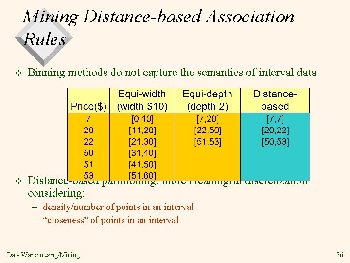
Mining Distance-based Association Rules v Binning methods do not capture the semantics of interval data v Distance-based partitioning, more meaningful discretization considering: – density/number of points in an interval – “closeness” of points in an interval Data Warehousing/Mining 36

DBMiner Examples v Show Examples 12 - 14 Data Warehousing/Mining 37

Interestingness Measurements v Objective measures Two popular measurements: support and confidence v Subjective measures (Silberschatz & Tuzhilin, KDD 95) A rule (pattern) is interesting i it is unexpected (surprising to the user); and/or actionable (the user can do something with it) Data Warehousing/Mining 38

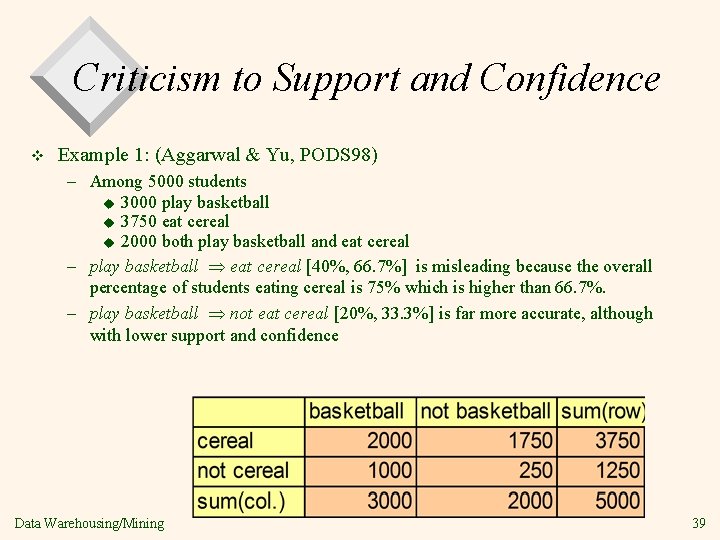
Criticism to Support and Confidence v Example 1: (Aggarwal & Yu, PODS 98) – Among 5000 students u 3000 play basketball u 3750 eat cereal u 2000 both play basketball and eat cereal – play basketball eat cereal [40%, 66. 7%] is misleading because the overall percentage of students eating cereal is 75% which is higher than 66. 7%. – play basketball not eat cereal [20%, 33. 3%] is far more accurate, although with lower support and confidence Data Warehousing/Mining 39

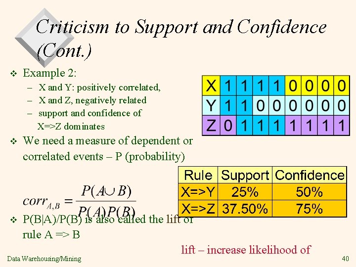
Criticism to Support and Confidence (Cont. ) v Example 2: – X and Y: positively correlated, – X and Z, negatively related – support and confidence of X=>Z dominates v We need a measure of dependent or correlated events – P (probability) v P(B|A)/P(B) is also called the lift of rule A => B lift – increase likelihood of Data Warehousing/Mining 40

Constraint-Based Mining v Interactive, exploratory mining giga-bytes of data? – Could it be real? — Making good use of constraints! v What kinds of constraints can be used in mining? – Knowledge type constraint: classification, association, etc. – Data constraint: SQL-like queries u Find product pairs sold together in Vancouver in Dec. ’ 98. – Dimension/level constraints: u in relevance to region, price, brand, customer category. – Rule constraints u small sales (price < $10) triggers big sales (sum > $200). – Interestingness constraints: u strong rules (min_support 3%, min_confidence 60%). Data Warehousing/Mining 41

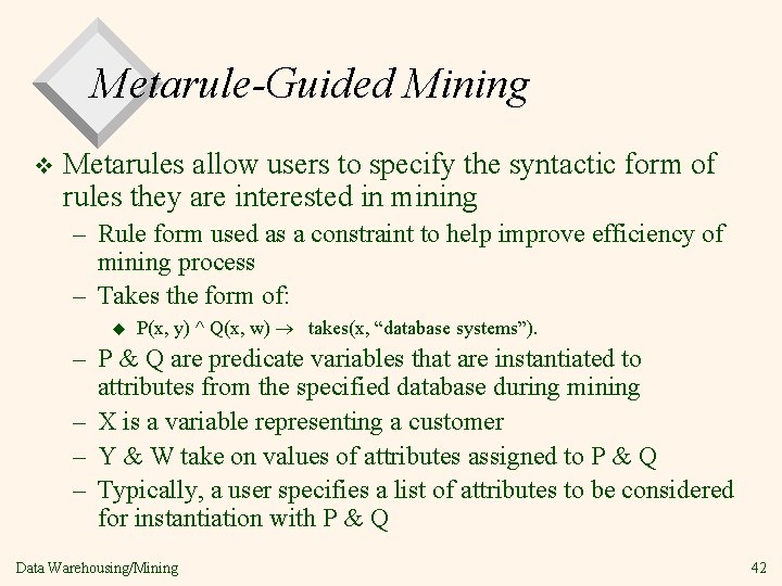
Metarule-Guided Mining v Metarules allow users to specify the syntactic form of rules they are interested in mining – Rule form used as a constraint to help improve efficiency of mining process – Takes the form of: u P(x, y) ^ Q(x, w) ® takes(x, “database systems”). – P & Q are predicate variables that are instantiated to attributes from the specified database during mining – X is a variable representing a customer – Y & W take on values of attributes assigned to P & Q – Typically, a user specifies a list of attributes to be considered for instantiation with P & Q Data Warehousing/Mining 42

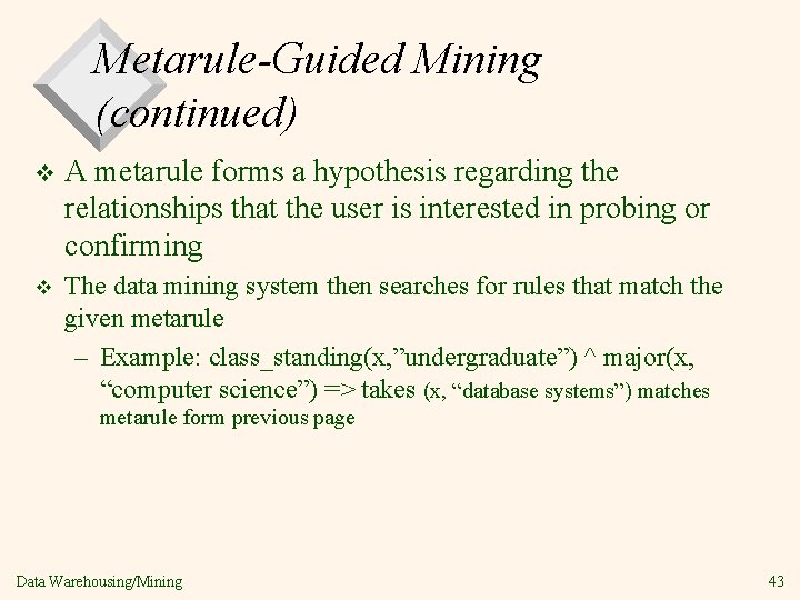
Metarule-Guided Mining (continued) v A metarule forms a hypothesis regarding the relationships that the user is interested in probing or confirming v The data mining system then searches for rules that match the given metarule – Example: class_standing(x, ”undergraduate”) ^ major(x, “computer science”) => takes (x, “database systems”) matches metarule form previous page Data Warehousing/Mining 43

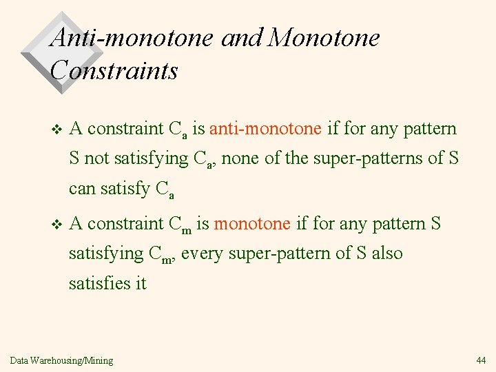
Anti-monotone and Monotone Constraints v A constraint Ca is anti-monotone if for any pattern S not satisfying Ca, none of the super-patterns of S can satisfy Ca v A constraint Cm is monotone if for any pattern S satisfying Cm, every super-pattern of S also satisfies it Data Warehousing/Mining 44

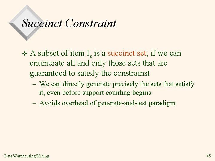
Succinct Constraint v A subset of item Is is a succinct set, set if we can enumerate all and only those sets that are guaranteed to satisfy the constrainst – We can directly generate precisely the sets that satisfy it, even before support counting begins – Avoids overhead of generate-and-test paradigm Data Warehousing/Mining 45

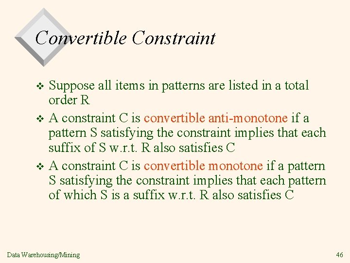
Convertible Constraint Suppose all items in patterns are listed in a total order R v A constraint C is convertible anti-monotone if a pattern S satisfying the constraint implies that each suffix of S w. r. t. R also satisfies C v A constraint C is convertible monotone if a pattern S satisfying the constraint implies that each pattern of which S is a suffix w. r. t. R also satisfies C v Data Warehousing/Mining 46

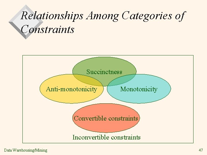
Relationships Among Categories of Constraints Succinctness Anti-monotonicity Monotonicity Convertible constraints Inconvertible constraints Data Warehousing/Mining 47

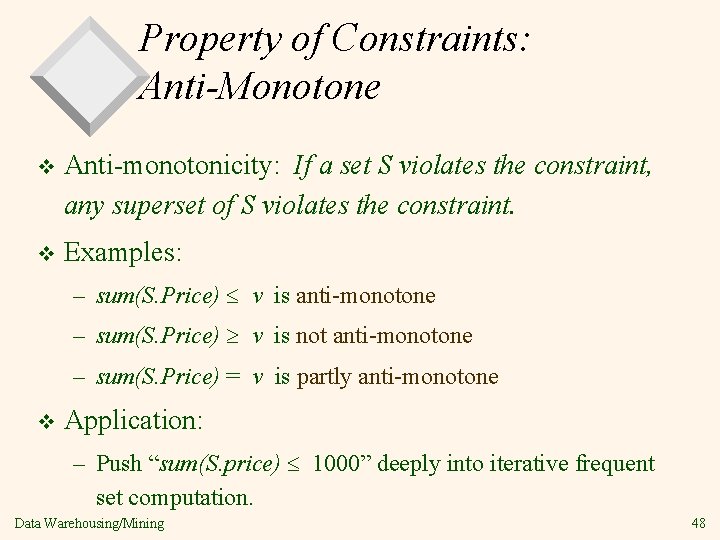
Property of Constraints: Anti-Monotone v Anti-monotonicity: If a set S violates the constraint, any superset of S violates the constraint. v Examples: – sum(S. Price) v is anti-monotone – sum(S. Price) v is not anti-monotone – sum(S. Price) = v is partly anti-monotone v Application: – Push “sum(S. price) 1000” deeply into iterative frequent set computation. Data Warehousing/Mining 48

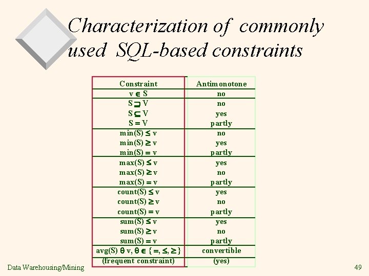
Characterization of commonly used SQL-based constraints Data Warehousing/Mining Constraint v S S V S V min(S) v max(S) v count(S) v sum(S) v avg(S) v, { , , } (frequent constraint) Antimonotone no no yes partly yes no partly convertible (yes) 49

Summary v Association rule mining – probably the most significant contribution from the database community in KDD – A large number of papers have been published v An interesting research direction – Association analysis in other types of data: spatial data, multimedia data, time series data, etc. Data Warehousing/Mining 50

Project Due - Thursday, May 13, 2004 v Look at Spring 04_Project. doc v Data Warehousing/Mining 51