CSE 221 Algorithms and Data Structures Lecture 8

CSE 221: Algorithms and Data Structures Lecture #8 What do you get when you put too many pigeons in one hole? Pigeon Hash Steve Wolfman 2009 W 1

Learning Goals After this unit, you should be able to: • Define various forms of the pigeonhole principle; recognize and solve the specific types of counting and hashing problems to which they apply. • Provide examples of the types of problems that can benefit from a hash data structure. • Compare and contrast open addressing and chaining. • Evaluate collision resolution policies. • Describe the conditions under which hashing can degenerate from O(1) expected complexity to O(n). • Identify the types of search problems that do not benefit from hashing (e. g. range searching) and explain why. • Manipulate data in hash structures both irrespective of implementation and also within a given implementation. 2

Today’s Outline • • • Constant-Time Dictionaries? Hash Table Outline Hash Functions Collisions and the Pigeonhole Principle Collision Resolution: – Chaining – Open-Addressing

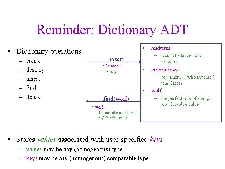
Reminder: Dictionary ADT • • Dictionary operations – – – create destroy insert find delete – would be tastier with brownies insert • brownies - tasty midterm • prog-project – so painful… who invented templates? • find(wolf) • wolf - the perfect mix of oomph wolf – the perfect mix of oomph and Scrabble value • Stores values associated with user-specified keys – values may be any (homogenous) type – keys may be any (homogenous) comparable type

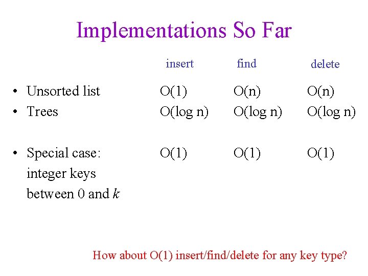
Implementations So Far insert find delete • Unsorted list • Trees O(1) O(log n) O(n) O(log n) • Special case: integer keys between 0 and k O(1) How about O(1) insert/find/delete for any key type?

Hash Table Goal 0 “Vicki” We can do: We want to do: 1 a[2] = “Andrew” 2 “Dan” a[“Steve”] = “Andrew” Andrew “Steve” Andrew “Shervin” 3 “Ben” … … k-1 “Martin”

Today’s Outline • • • Constant-Time Dictionaries? Hash Table Outline Hash Functions Collisions and the Pigeonhole Principle Collision Resolution: – Chaining – Open-Addressing

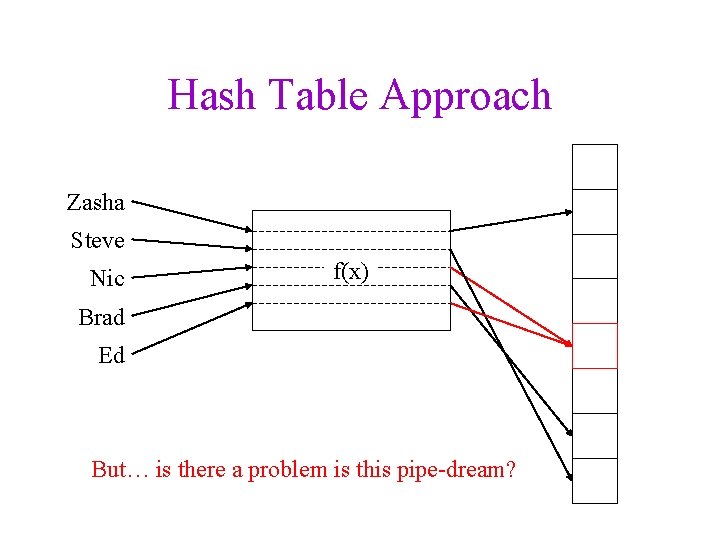
Hash Table Approach Zasha Steve Nic f(x) Brad Ed But… is there a problem is this pipe-dream?

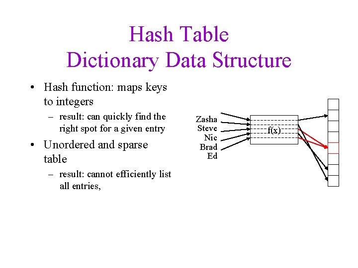
Hash Table Dictionary Data Structure • Hash function: maps keys to integers – result: can quickly find the right spot for a given entry • Unordered and sparse table – result: cannot efficiently list all entries, Zasha Steve Nic Brad Ed f(x)

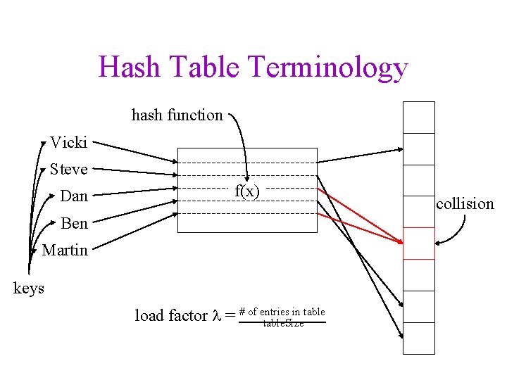
Hash Table Terminology hash function Vicki Steve Dan f(x) Ben Martin keys in table load factor = # of entries table. Size collision

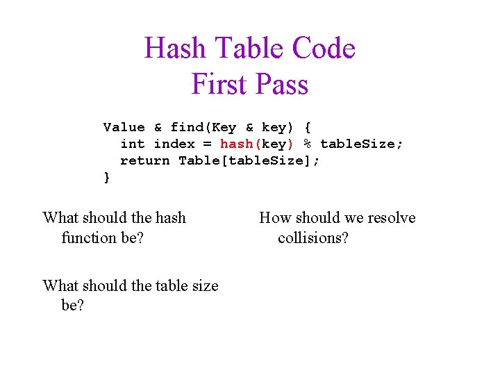
Hash Table Code First Pass Value & find(Key & key) { int index = hash(key) % table. Size; return Table[table. Size]; } What should the hash function be? What should the table size be? How should we resolve collisions?

Today’s Outline • • • Constant-Time Dictionaries? Hash Table Outline Hash Functions Collisions and the Pigeonhole Principle Collision Resolution: – Chaining – Open-Addressing

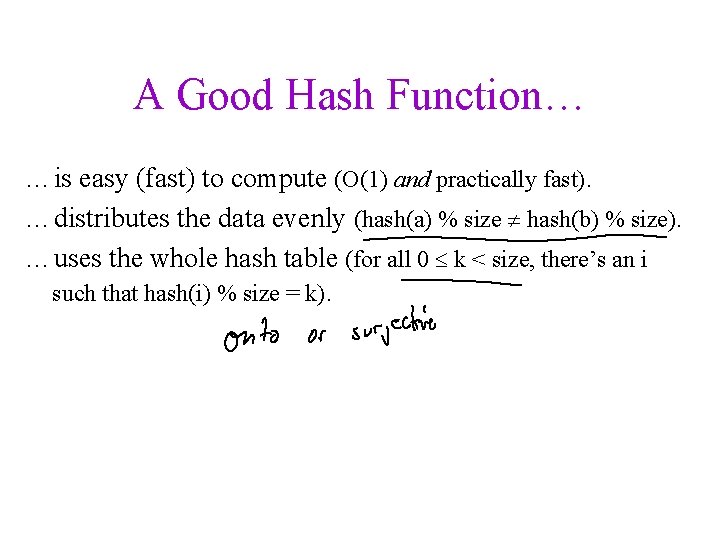
A Good Hash Function… …is easy (fast) to compute (O(1) and practically fast). …distributes the data evenly (hash(a) % size hash(b) % size). …uses the whole hash table (for all 0 k < size, there’s an i such that hash(i) % size = k).

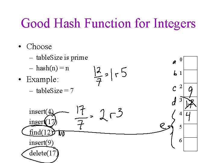
Good Hash Function for Integers • Choose – table. Size is prime – hash(n) = n • Example: – table. Size = 7 0 1 2 3 insert(4) insert(17) find(12) insert(9) delete(17) 4 5 6

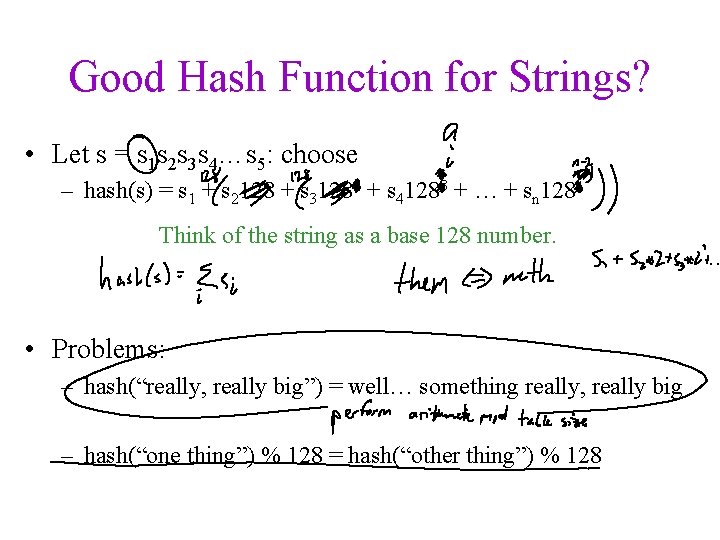
Good Hash Function for Strings? • Let s = s 1 s 2 s 3 s 4…s 5: choose – hash(s) = s 1 + s 2128 + s 31282 + s 41283 + … + sn 128 n Think of the string as a base 128 number. • Problems: – hash(“really, really big”) = well… something really, really big – hash(“one thing”) % 128 = hash(“other thing”) % 128

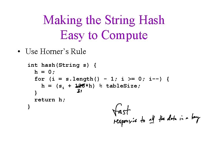
Making the String Hash Easy to Compute • Use Horner’s Rule int hash(String s) { h = 0; for (i = s. length() - 1; i >= 0; i--) { h = (si + 128*h) % table. Size; } return h; }

Making the String Hash Cause Few Conflicts • Ideas?

Hash Function Summary • Goals of a hash function – – reproducible mapping from key to table entry evenly distribute keys across the table separate commonly occurring keys (neighboring keys? ) complete quickly • Sample hash functions: – – – h(n) = n % size h(n) = string as base 128 number % size Multiplication hash: compute percentage through the table Universal hash function #1: dot product with random vector Universal hash function #2: next pseudo-random number

How to Design a Hash Function • Know what your keys are or • Study how your keys are distributed. • Try to include all important information in a key in the construction of its hash. • Try to make “neighboring” keys hash to very different places. • Prune the features used to create the hash until it runs “fast enough” (very application dependent).

Today’s Outline • • • Constant-Time Dictionaries? Hash Table Outline Hash Functions Collisions and the Pigeonhole Principle Collision Resolution: – Chaining – Open-Addressing

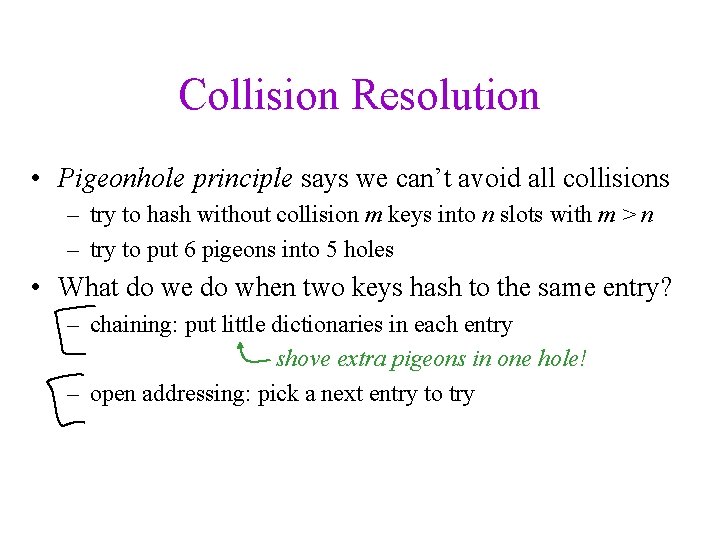
Collisions • Pigeonhole principle says we can’t avoid all collisions – try to hash without collision m keys into n slots with m > n – try to put 6 pigeons into 5 holes

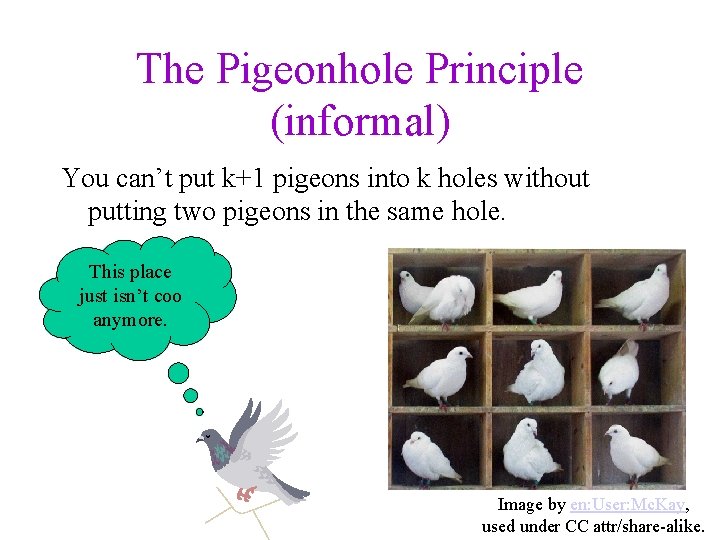
The Pigeonhole Principle (informal) You can’t put k+1 pigeons into k holes without putting two pigeons in the same hole. This place just isn’t coo anymore. Image by en: User: Mc. Kay, used under CC attr/share-alike.

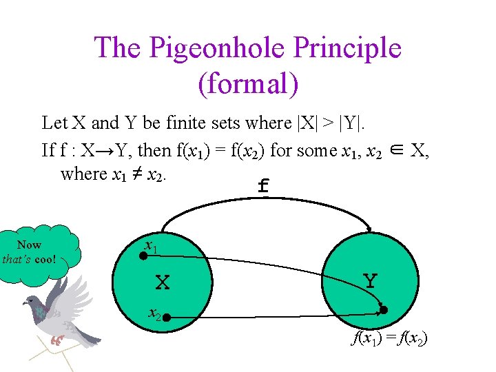
The Pigeonhole Principle (formal) Let X and Y be finite sets where |X| > |Y|. If f : X→Y, then f(x 1) = f(x 2) for some x 1, x 2 ∈ X, where x 1 ≠ x 2. f Now that’s coo! x 1 X Y x 2 f(x 1) = f(x 2)

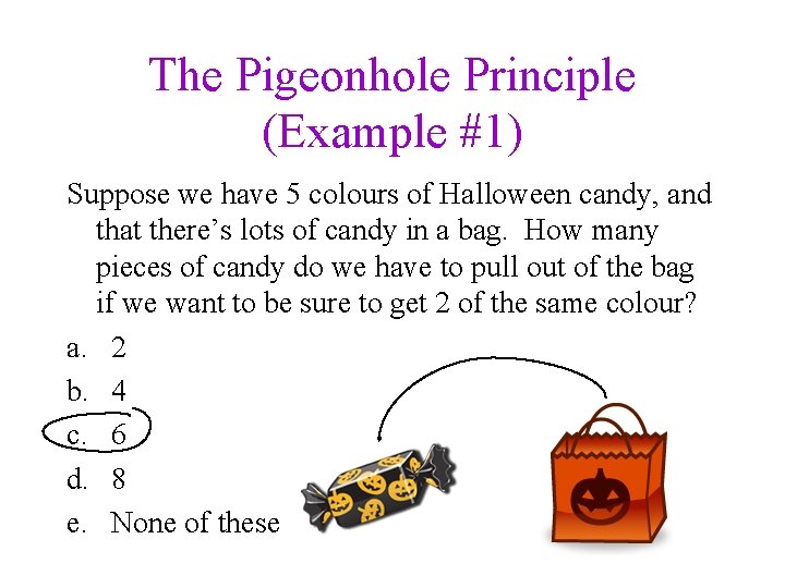
The Pigeonhole Principle (Example #1) Suppose we have 5 colours of Halloween candy, and that there’s lots of candy in a bag. How many pieces of candy do we have to pull out of the bag if we want to be sure to get 2 of the same colour? a. 2 b. 4 c. 6 d. 8 e. None of these

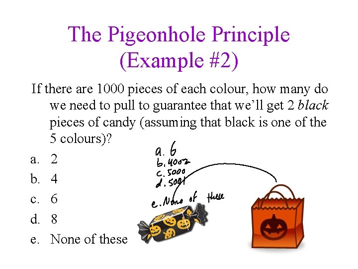
The Pigeonhole Principle (Example #2) If there are 1000 pieces of each colour, how many do we need to pull to guarantee that we’ll get 2 black pieces of candy (assuming that black is one of the 5 colours)? a. 2 b. 4 c. 6 d. 8 e. None of these

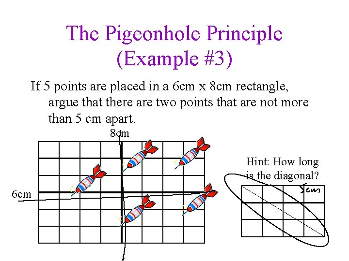
The Pigeonhole Principle (Example #3) If 5 points are placed in a 6 cm x 8 cm rectangle, argue that there are two points that are not more than 5 cm apart. 8 cm Hint: How long is the diagonal? 6 cm

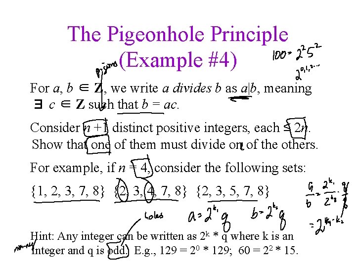
The Pigeonhole Principle (Example #4) For a, b ∈ Z, we write a divides b as a|b, meaning ∃ c ∈ Z such that b = ac. Consider n +1 distinct positive integers, each ≤ 2 n. Show that one of them must divide on of the others. For example, if n = 4, consider the following sets: {1, 2, 3, 7, 8} {2, 3, 4, 7, 8} {2, 3, 5, 7, 8} Hint: Any integer can be written as 2 k * q where k is an integer and q is odd. E. g. , 129 = 20 * 129; 60 = 22 * 15.

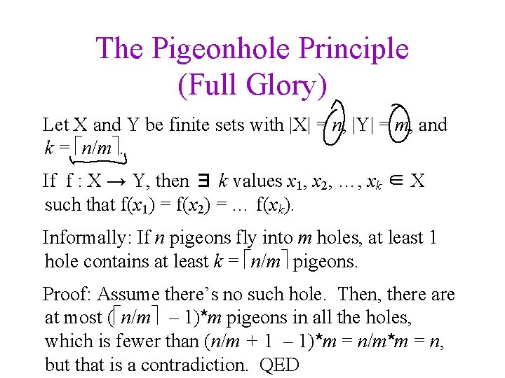
The Pigeonhole Principle (Full Glory) Let X and Y be finite sets with |X| = n, |Y| = m, and k = n/m. If f : X → Y, then ∃ k values x 1, x 2, …, xk ∈ X such that f(x 1) = f(x 2) = … f(xk). Informally: If n pigeons fly into m holes, at least 1 hole contains at least k = n/m pigeons. Proof: Assume there’s no such hole. Then, there at most ( n/m – 1)*m pigeons in all the holes, which is fewer than (n/m + 1 – 1)*m = n/m*m = n, but that is a contradiction. QED

Today’s Outline • • • Constant-Time Dictionaries? Hash Table Outline Hash Functions Collisions and the Pigeonhole Principle Collision Resolution: – Chaining – Open-Addressing

Collision Resolution • Pigeonhole principle says we can’t avoid all collisions – try to hash without collision m keys into n slots with m > n – try to put 6 pigeons into 5 holes • What do we do when two keys hash to the same entry? – chaining: put little dictionaries in each entry shove extra pigeons in one hole! – open addressing: pick a next entry to try

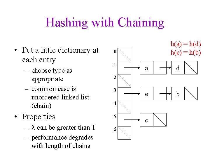
Hashing with Chaining • Put a little dictionary at each entry – choose type as appropriate – common case is unordered linked list (chain) • Properties – can be greater than 1 – performance degrades with length of chains h(a) = h(d) h(e) = h(b) 0 1 a d e b 2 3 4 5 6 c

Chaining Code Dictionary & find. Bucket(const Key & k) { return table[hash(k)%table. size]; } void insert(const Key & k, const Value & v) { find. Bucket(k). insert(k, v); } void delete(const Key & k) { find. Bucket(k). delete(k); } Value & find(const Key & k) { return find. Bucket(k). find(k); }

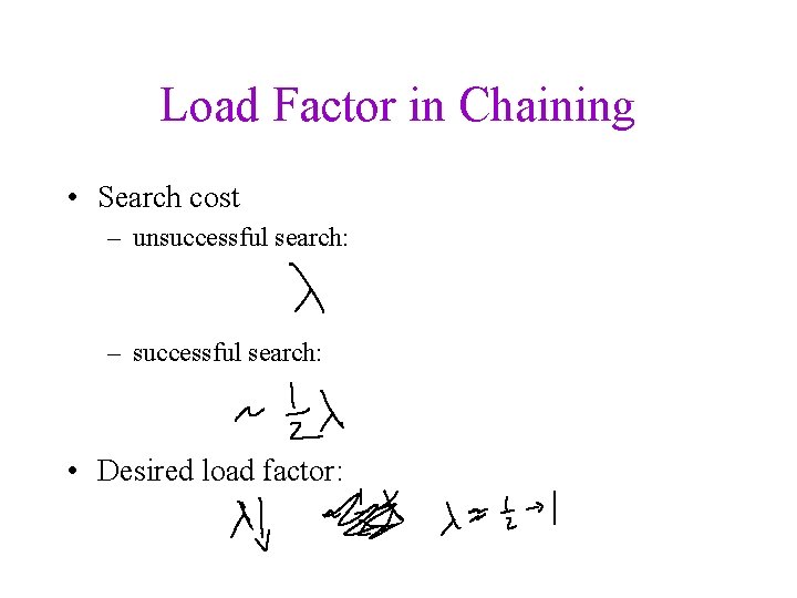
Load Factor in Chaining • Search cost – unsuccessful search: – successful search: • Desired load factor:

Today’s Outline • • • Constant-Time Dictionaries? Hash Table Outline Hash Functions Collisions and the Pigeonhole Principle Collision Resolution: – Chaining – Open-Addressing

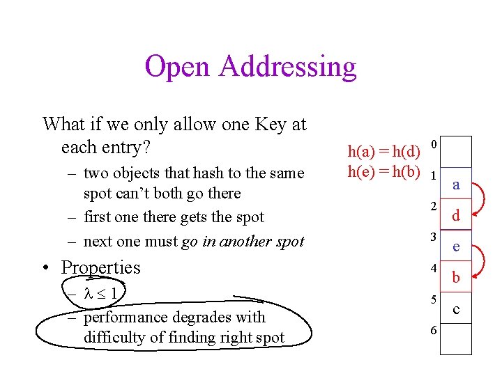
Open Addressing What if we only allow one Key at each entry? – two objects that hash to the same spot can’t both go there – first one there gets the spot – next one must go in another spot • Properties – 1 – performance degrades with difficulty of finding right spot h(a) = h(d) h(e) = h(b) 0 1 2 3 4 5 6 a d e b c

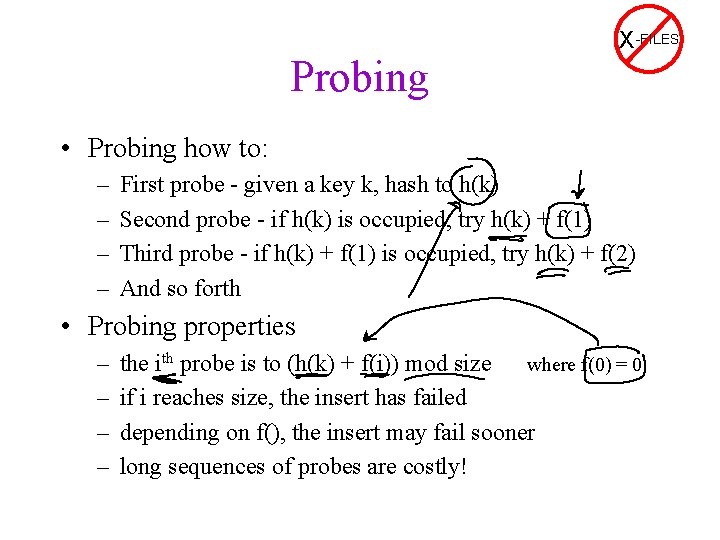
Probing X-FILES • Probing how to: – – First probe - given a key k, hash to h(k) Second probe - if h(k) is occupied, try h(k) + f(1) Third probe - if h(k) + f(1) is occupied, try h(k) + f(2) And so forth • Probing properties – – the ith probe is to (h(k) + f(i)) mod size where f(0) = 0 if i reaches size, the insert has failed depending on f(), the insert may fail sooner long sequences of probes are costly!

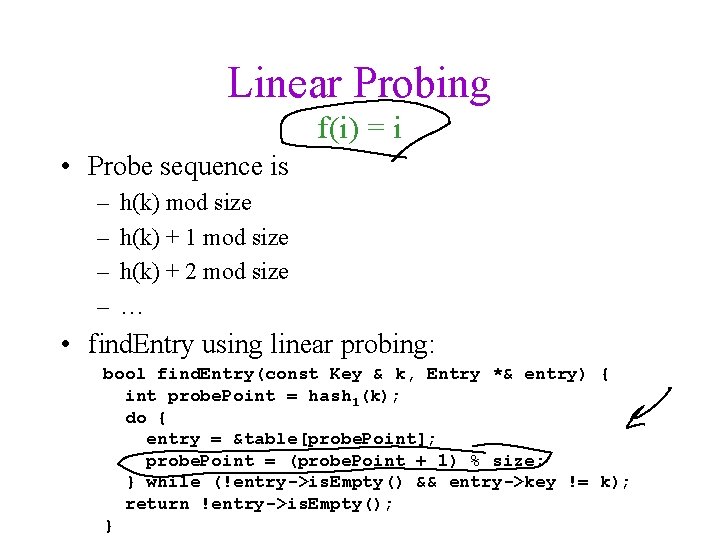
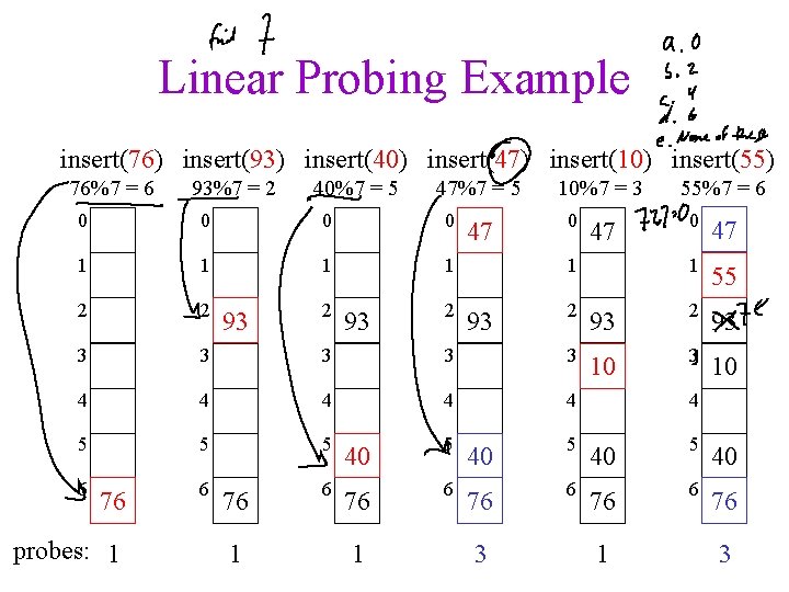
Linear Probing f(i) = i • Probe sequence is – – h(k) mod size h(k) + 1 mod size h(k) + 2 mod size … • find. Entry using linear probing: bool find. Entry(const Key & k, Entry *& entry) { int probe. Point = hash 1(k); do { entry = &table[probe. Point]; probe. Point = (probe. Point + 1) % size; } while (!entry->is. Empty() && entry->key != k); return !entry->is. Empty(); }

Linear Probing Example insert(76) insert(93) insert(40) insert(47) insert(10) insert(55) 76%7 = 6 93%7 = 2 40%7 = 5 47%7 = 5 0 0 1 1 2 2 3 3 3 4 4 5 5 6 76 probes: 1 6 93 76 1 2 0 47 1 55%7 = 6 0 47 1 55 2 93 3 3 10 4 4 5 40 6 76 93 1 2 47 10%7 = 3 93 3 1 3

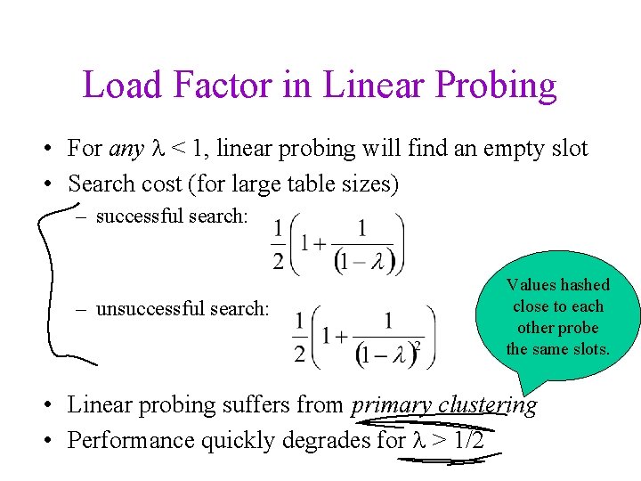
Load Factor in Linear Probing • For any < 1, linear probing will find an empty slot • Search cost (for large table sizes) – successful search: – unsuccessful search: Values hashed close to each other probe the same slots. • Linear probing suffers from primary clustering • Performance quickly degrades for > 1/2

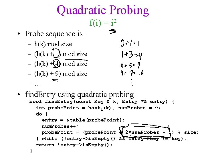
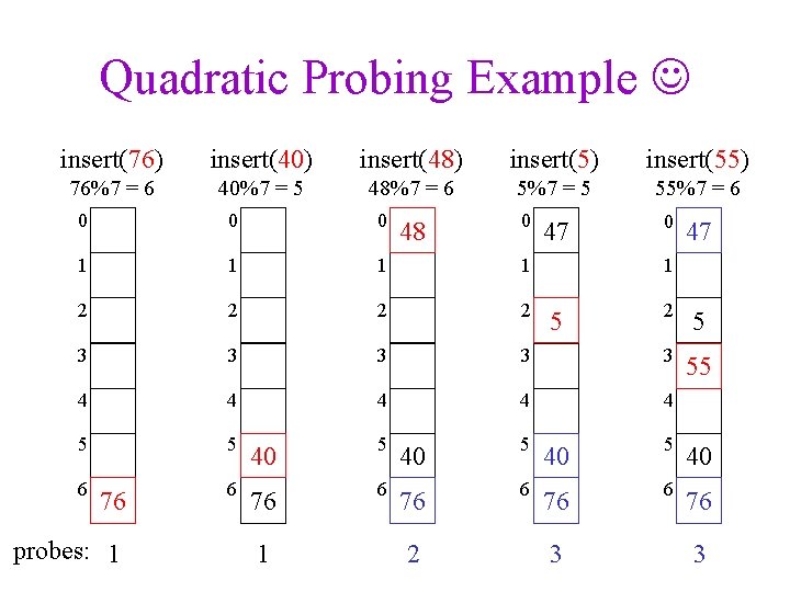
Quadratic Probing f(i) = i 2 • Probe sequence is – – – h(k) mod size (h(k) + 1) mod size (h(k) + 4) mod size (h(k) + 9) mod size … • find. Entry using quadratic probing: bool find. Entry(const Key & k, Entry *& entry) { int probe. Point = hash 1(k), num. Probes = 0; do { entry = &table[probe. Point]; num. Probes++; probe. Point = (probe. Point + 2*num. Probes - 1) % size; } while (!entry->is. Empty() && entry->key != key); return !entry->is. Empty(); }

Quadratic Probing Example insert(76) insert(40) insert(48) insert(55) 76%7 = 6 40%7 = 5 48%7 = 6 5%7 = 5 55%7 = 6 0 0 0 1 1 2 2 3 3 3 4 4 5 5 6 6 76 probes: 1 48 0 47 1 2 5 3 3 55 4 40 5 40 76 6 76 1 2 5 3 3

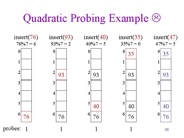
Quadratic Probing Example insert(76) insert(93) insert(40) insert(35) insert(47) 76%7 = 6 93%7 = 2 40%7 = 5 35%7 = 0 47%7 = 5 0 0 1 1 2 2 3 3 3 4 4 4 5 5 5 40 6 76 probes: 1 6 93 76 1 2 93 1 2 35 0 35 1 93 1 2 93

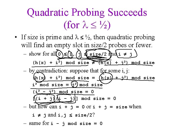
Quadratic Probing Succeeds (for ½) • If size is prime and ½, then quadratic probing will find an empty slot in size/2 probes or fewer. – show for all 0 i, j size/2 and i j (h(x) + i 2) mod size (h(x) + j 2) mod size – by contradiction: suppose that for some i, j: (h(x) + i 2) mod size = (h(x) + j 2) mod size i 2 mod size = j 2 mod size (i 2 - j 2) mod size = 0 [(i + j)(i - j)] mod size = 0 – but how can i + j = 0 or i + j = size when i j and i, j size/2? – same for i - j mod size = 0

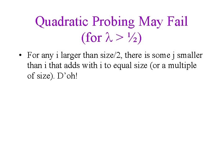
Quadratic Probing May Fail (for > ½) • For any i larger than size/2, there is some j smaller than i that adds with i to equal size (or a multiple of size). D’oh!

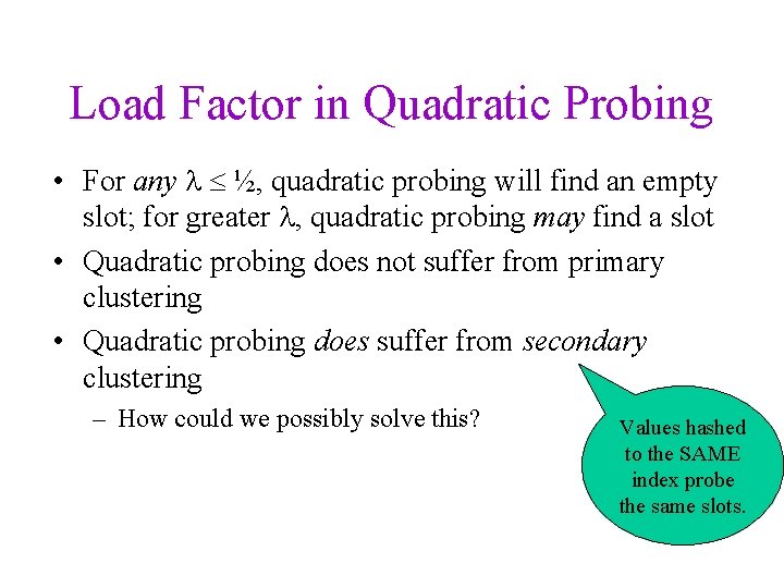
Load Factor in Quadratic Probing • For any ½, quadratic probing will find an empty slot; for greater , quadratic probing may find a slot • Quadratic probing does not suffer from primary clustering • Quadratic probing does suffer from secondary clustering – How could we possibly solve this? Values hashed to the SAME index probe the same slots.

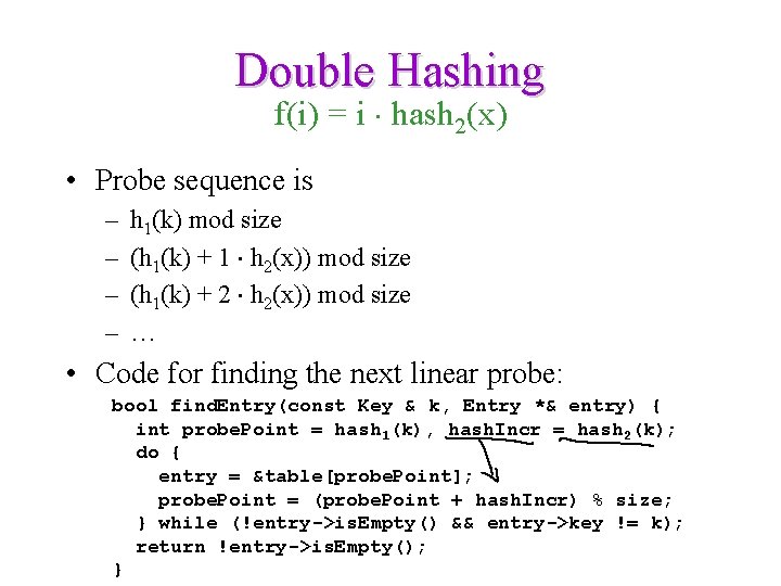
Double Hashing f(i) = i hash 2(x) • Probe sequence is – – h 1(k) mod size (h 1(k) + 1 h 2(x)) mod size (h 1(k) + 2 h 2(x)) mod size … • Code for finding the next linear probe: bool find. Entry(const Key & k, Entry *& entry) { int probe. Point = hash 1(k), hash. Incr = hash 2(k); do { entry = &table[probe. Point]; probe. Point = (probe. Point + hash. Incr) % size; } while (!entry->is. Empty() && entry->key != k); return !entry->is. Empty(); }

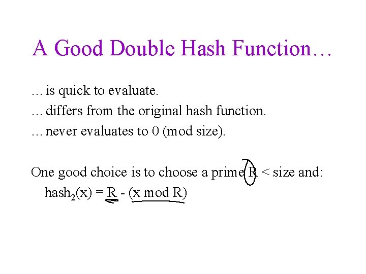
A Good Double Hash Function… …is quick to evaluate. …differs from the original hash function. …never evaluates to 0 (mod size). One good choice is to choose a prime R < size and: hash 2(x) = R - (x mod R)

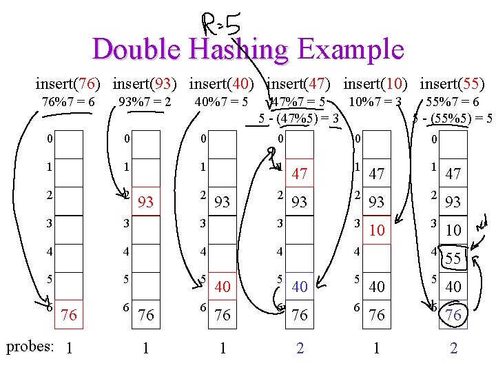
Double Hashing Example insert(76) insert(93) insert(40) insert(47) insert(10) insert(55) 76%7 = 6 93%7 = 2 40%7 = 5 47%7 = 5 10%7 = 3 55%7 = 6 5 - (47%5) = 3 5 - (55%5) = 5 0 0 1 1 47 2 2 2 93 3 3 10 4 4 4 55 5 40 5 40 6 76 6 76 probes: 1 6 93 76 1 2 93 1 0 2 0 1 2

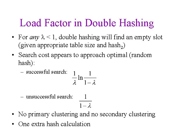
Load Factor in Double Hashing • For any < 1, double hashing will find an empty slot (given appropriate table size and hash 2) • Search cost appears to approach optimal (random hash): – successful search: – unsuccessful search: • No primary clustering and no secondary clustering • One extra hash calculation

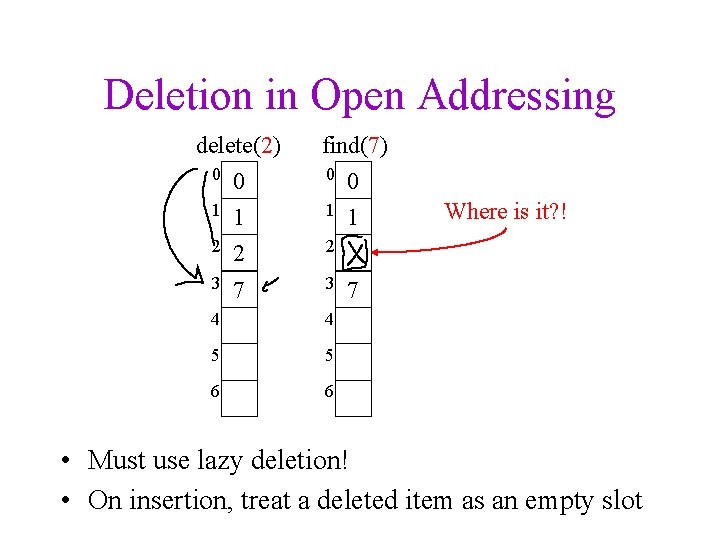
Deletion in Open Addressing delete(2) find(7) 0 0 1 1 2 2 2 3 7 3 4 4 5 5 6 6 Where is it? ! 7 • Must use lazy deletion! • On insertion, treat a deleted item as an empty slot

The Squished Pigeon Principle • An insert using open addressing cannot work with a load factor of 1 or more. • An insert using open addressing with quadratic probing may not work with a load factor of ½ or more. • Whether you use chaining or open addressing, large load factors lead to poor performance! • How can we relieve the pressure on the pigeons? Hint: think resizable arrays!

Rehashing • When the load factor gets “too large” (over a constant threshold on ), rehash all the elements into a new, larger table: – takes O(n), but amortized O(1) as long as we (just about) double table size on the resize – spreads keys back out, may drastically improve performance – gives us a chance to retune parameterized hash functions – avoids failure for open addressing techniques – allows arbitrarily large tables starting from a small table – clears out lazily deleted items

To Do • Start HW#3 (out soon) • Start Project 4 (out soon… our last project!) • Read Epp Section 7. 3 and Koffman & Wolfgang Chapter 9

Coming Up • Counting. What? Counting? ! Yes, counting, like: If you want to find the average depth of a binary tree as a function of its size, you have to count how many different binary trees there are with n nodes. Or: How many different ways are there to answer the question “How many fingers am I holding up, and which ones are they? ”

Extra Slides: Some Other Hashing Methods These are parameterized methods, which is handy if you know the keys in advance. In that case, you can randomly set the parameters a few times and pick a hash function that performs well. (Would that ever happen? How about when building a spell-check dictionary? )

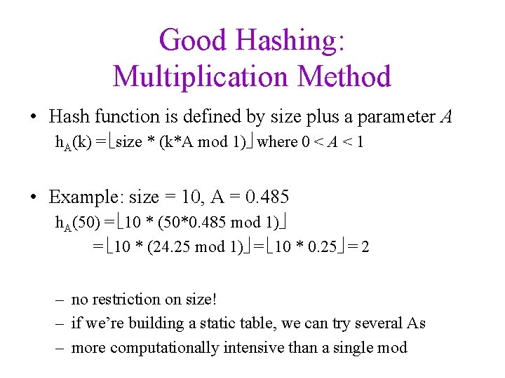
Good Hashing: Multiplication Method • Hash function is defined by size plus a parameter A h. A(k) = size * (k*A mod 1) where 0 < A < 1 • Example: size = 10, A = 0. 485 h. A(50) = 10 * (50*0. 485 mod 1) = 10 * (24. 25 mod 1) = 10 * 0. 25 = 2 – no restriction on size! – if we’re building a static table, we can try several As – more computationally intensive than a single mod

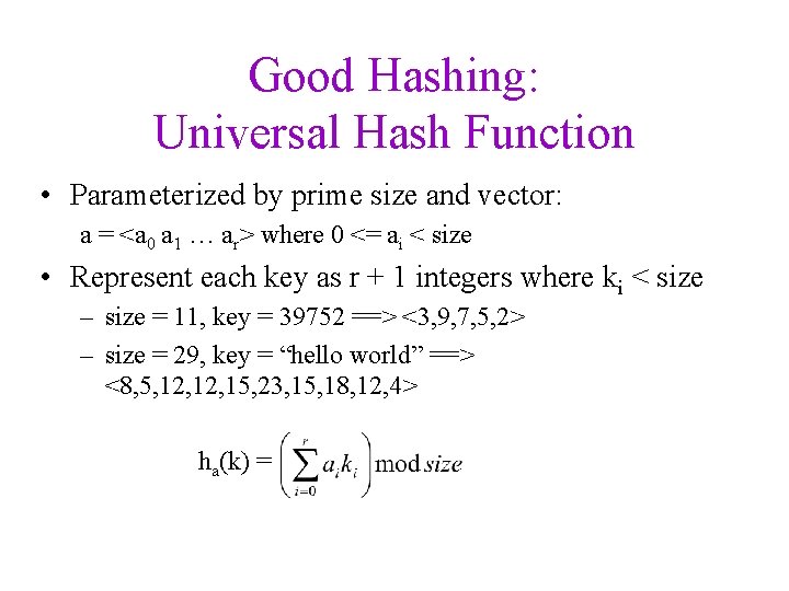
Good Hashing: Universal Hash Function • Parameterized by prime size and vector: a = <a 0 a 1 … ar> where 0 <= ai < size • Represent each key as r + 1 integers where ki < size – size = 11, key = 39752 ==> <3, 9, 7, 5, 2> – size = 29, key = “hello world” ==> <8, 5, 12, 15, 23, 15, 18, 12, 4> ha(k) =

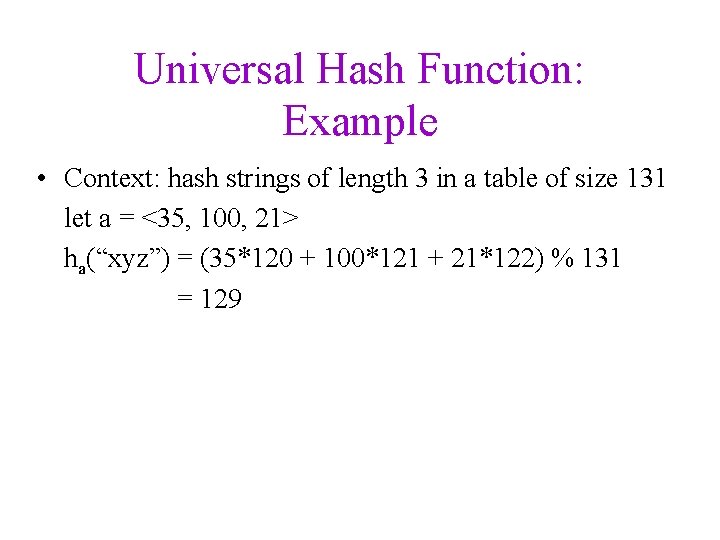
Universal Hash Function: Example • Context: hash strings of length 3 in a table of size 131 let a = <35, 100, 21> ha(“xyz”) = (35*120 + 100*121 + 21*122) % 131 = 129

Universal Hash Function • Strengths: – works on any type as long as you can form ki’s – if we’re building a static table, we can try many a’s – a random a has guaranteed good properties no matter what we’re hashing • Weaknesses – must choose prime table size larger than any ki

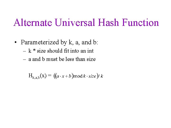
Alternate Universal Hash Function • Parameterized by k, a, and b: – k * size should fit into an int – a and b must be less than size Hk, a, b(x) =

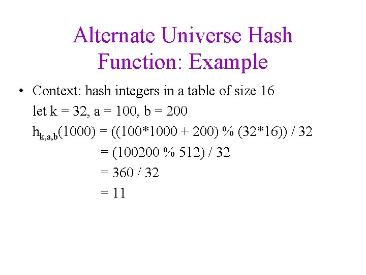
Alternate Universe Hash Function: Example • Context: hash integers in a table of size 16 let k = 32, a = 100, b = 200 hk, a, b(1000) = ((100*1000 + 200) % (32*16)) / 32 = (100200 % 512) / 32 = 360 / 32 = 11

Universal Hash Function • Strengths: – if we’re building a static table, we can try many a’s – random a, b has guaranteed good properties no matter what we’re hashing – can choose any size table – very efficient if k and size are powers of 2 • Weaknesses – still need to turn non-integer keys into integers