CS 655 Distributed Ray Tracing Distributed Ray Tracing

CS 655 Distributed Ray Tracing

Distributed Ray Tracing What is distributed ray tracing? § Distributed ray tracing is not ray tracing on a distributed system. § Distributed ray tracing is a ray tracing method based on randomly distributed oversampling to reduce aliasing artifacts in rendered images. § Also called “distribution ray tracing” or “stochastic ray tracing” § (The images in this presentation are from Andrew G. Zaferakis, Aneesh Naman, Allen Martin, Daqing Xue, Henrik Wann Jensen, and Jinho Lee)

Distributed Ray Tracing • Idea: Introduce noise into the ray tracer to minimize visual artifacts such as aliasing, perfect reflections, etc. • Stocastically distribute rays over: § § § Space – antialiases the image Reflection angle – produces glossy reflections Transmission angle – produces translucency Shadow ray – produces soft shadows (penumbra) Lens area – produces depth of field Time – produces motion blur

Antialiasing • The human eye samples using a Poisson disk distribution: • A finite number of photoreceptors • Cones in the eye are distributed stochastically, but such that no two cones are closer than a certain distance

Antialiasing • We can apply this approach to ray tracing § Send out rays stochastically, but such that they maintain a Poisson disk distribution • This reduces aliasing, but is expensive to compute • However, we can approximate a Poisson disk distribution fairly quickly • Idea: begin with a regular grid • Jitter the ray locations slightly within the grid

Uniform Sampling Prone to aliasing in the image

Jittered Sampling Antialiases the image

Jittered Sampling • Approximates a Poisson disk distribution § Not exact, but much cheaper • Removes high frequencies • Introduces noise in place of high frequencies • Can still have problems § May leave large areas uncovered by samples § May have some areas with more samples than necessary

Improved Jittered Sampling • To improve the image further, send out multiple jittered rays per pixel Similarly for all other pixels • Make the number of sub-pixels easily changeable – start small then increase as you are confident your raytracer works.

Standard Ray Tracing • No antialiasing

Distributed Ray Tracing • With antialiasing

Standard Ray Tracing - detail • No antialiasing

Distributed Ray Tracing - detail • With antialiasing

Glossy Reflections • We can use the concept of ray jittering to produce glossiness (blurred reflections) • Tracing a ray based on perfect reflection angle produces sharp reflections N I R

Glossy Reflections • We can create a blurred reflection by sending out jittered rays about the reflection ray N I R Bound of jittered reflection rays

Glossy Reflections • This has the effect of “blurring” the reflection • The exact reflection vector is computed, then slightly jittered from the original direction • The jittered ray may hit an entirely different object than the one hit by the true reflection ray • This gives a smoothly blurred reflection

Reflections – Standard Ray Tracer • Perfect reflection

Reflections – Distributed Ray Tracer • 10 distributed rays

Reflections – Distributed Ray Tracer • 20 distributed rays

Reflections – Distributed Ray Tracer • 50 distributed rays

Standard Ray Tracing • Perfect reflections

Glossy reflections • 4 rays

Glossy reflections • 16 rays

Glossy reflections • 64 rays

Translucency • We can also apply the concept of ray jittering to produce translucency (blurred transmissions) • Tracing a ray based on perfect transmission angle produces sharp transparencies N I T

Translucency N I • Jittering the rays about the actual transmission angle produces a blurred effect Bound of jittered reflection rays T

Transmissions – Standard Ray Tracer • Perfect transmission

Transmissions – Distributed Ray Tracer • 10 transmission rays

Transmissions – Distributed Ray Tracer • 20 transmission rays

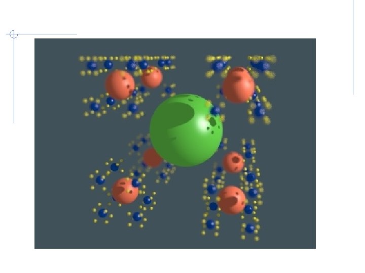
From Jia, Sun, and Xu

Soft Shadows • We have been simulating lights with point light sources • This produces hard shadows Point light source -hard shadow

Soft Shadows • Lights in the real world are not point light sources, thus the shadows are not sharp Area light source umbra Area light source -soft shadow penumbra

Soft Shadows • The penumbra is the portion of the shadow resulting from partially obscured lights Area light source • To simulate penumbra: § § § Send out multiple shadow rays from the intersection point to the area light source Jitter the rays according to the area light source The intensity of the surface point depends on the number of jittered rays that reach the light source Bounds of jittered shadow rays Occluding object Intersection point

Hard Shadows

Soft Shadows

Standard Ray Tracing • Hard shadows

Ray Tracing with an Area Light Source • Visible penumbra and umbra, but too distinct

Distributed Ray Tracing • 10 rays per pixel

Distributed Ray Tracing • 20 rays per pixel

Distributed Ray Tracing • 50 rays per pixel
 should have a fixed focal")
Depth of Field • Idea: the camera (or eye) should have a fixed focal length § Objects at that distance should be in focus § Objects closer or further away should not be in focus Lens Image Plane Focal Plane

Lens Properties D VD r P Vp Pf C F/n Object in Scene Lens Image Plane PD Focal Plane

Lens Properties F: n: F/n: Pf: P: Focal length aperture number lens diameter the focal point distance from lens to focal point Vp: distance from lens to image plane PD: a point not on the focal plane D: distance from lens to PD r: radius of cone for object at distance D C: circle of confusion D VD Vp C Image Plane Lens r P F/n Pf Focal Plane PD Object in Scene

Simulating a lens • Approach 1: § For an object located at PD, send out a group of jittered rays that lie within a cone of radius r How do we compute r? § This simulates a lens without actually having one, but isn’t very accurate §

Simulating a lens • Approach 2: Find the focal point 1. - Send a ray from the center of the lens (eye point) through the screen and follow it a distance P 2. Choose a jittered point on the lens 3. Trace a ray from that jittered point through the focal point 4. Return intensity information based on what that ray hits

Simulating a lens • Step 1 – determine the focal point by tracing a ray from the lens center through the pixel a distance P

Simulating a lens • Step 2 – Choose a jittered point on the lens New point

Simulating a lens • Step 3 – Trace the ray from the new point through the focal point

Simulating a lens • Step 4 – Return the intensity information

Depth of Field Example

Depth of Field Example From Alan Watt, “ 3 D Computer Graphics”

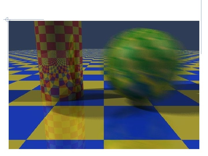
Motion Blur • Distribute rays over time § Static objects will not change § Moving objects will be blurred, depending on their velocity • How: § § Jitter the rays with respect to time Determine object positions at each of the jittered time values Send each ray with the objects positioned appropriately Combine the rays back into one to get the motion blurred object
")
Motion Blur Example (from Cook et. al. )

Summary of Distributed Ray Tracing • For each ray do: 1. Jitter the spatial screen location of the ray 2. Select a time for the ray and move the objects to that time Perform depth of field calculation: 3. a. b. 4. 5. 6. 7. Determine the focal point by sending a ray from the eye point (center of the lens) through the pixel, a distance P Determine a lens location by jittering the origin of the ray to a position on the lens Compute the intersection by sending the primary ray from the jittered location through the focal point Trace jittered reflection rays Trace jittered trasmission rays Trace jittered shadow rays

Summary of Distributed Ray Tracing Shadow Ray Reflected Ray Transmitted Ray
")
Distributed Ray Tracing (Cook et. al. )
- Slides: 58