Monte Carlo Path Tracing Today n Path tracing



- Slides: 32

Monte Carlo Path Tracing Today n Path tracing n Random walks and Markov chains n Eye vs. light ray tracing n Bidirectional ray tracing Next n Irradiance caching n Photon mapping CS 348 B Lecture 14 Pat Hanrahan, Spring 2005

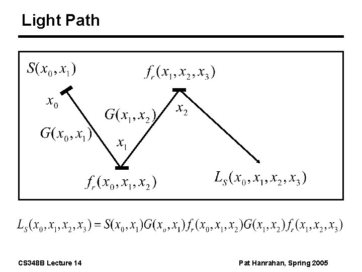
Light Path CS 348 B Lecture 14 Pat Hanrahan, Spring 2005

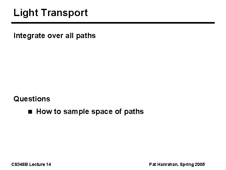
Light Transport Integrate over all paths Questions n How to sample space of paths CS 348 B Lecture 14 Pat Hanrahan, Spring 2005

Path Tracing

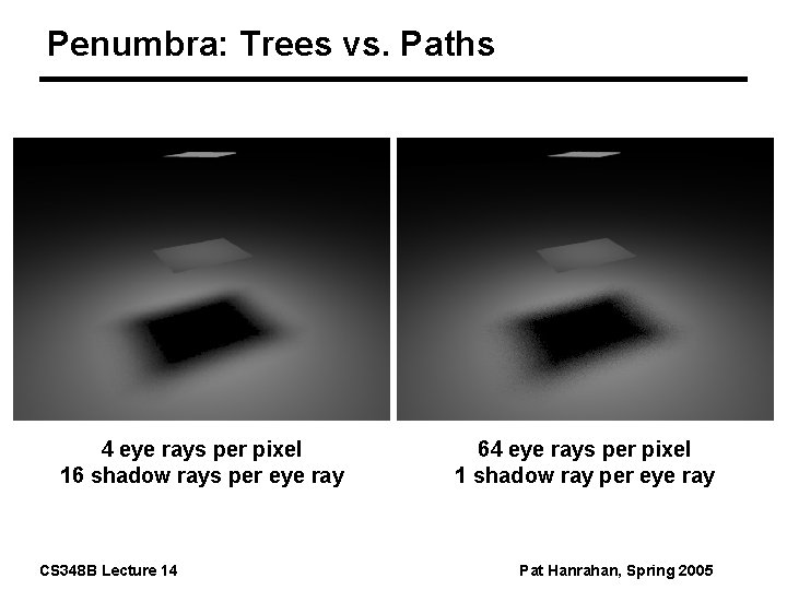
Penumbra: Trees vs. Paths 4 eye rays per pixel 16 shadow rays per eye ray CS 348 B Lecture 14 64 eye rays per pixel 1 shadow ray per eye ray Pat Hanrahan, Spring 2005

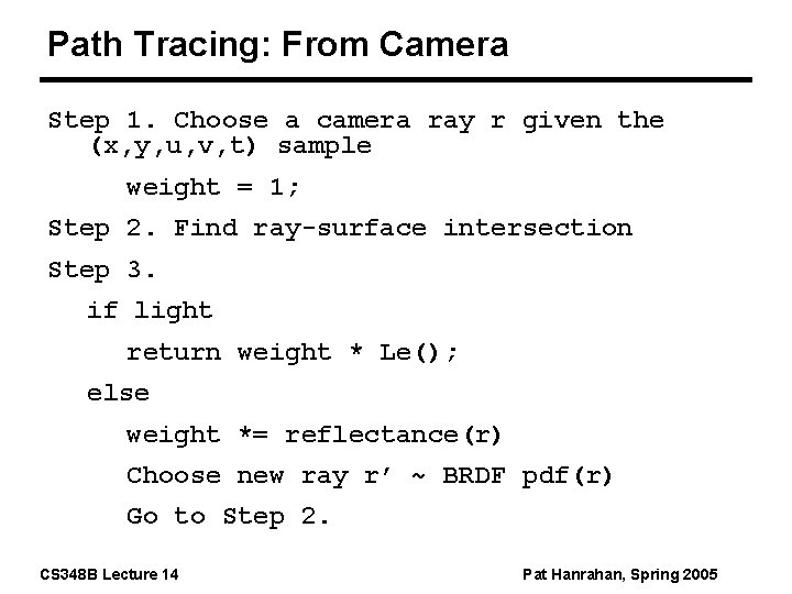
Path Tracing: From Camera Step 1. Choose a camera ray r given the (x, y, u, v, t) sample weight = 1; Step 2. Find ray-surface intersection Step 3. if light return weight * Le(); else weight *= reflectance(r) Choose new ray r’ ~ BRDF pdf(r) Go to Step 2. CS 348 B Lecture 14 Pat Hanrahan, Spring 2005

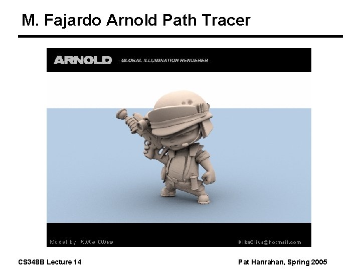
M. Fajardo Arnold Path Tracer CS 348 B Lecture 14 Pat Hanrahan, Spring 2005

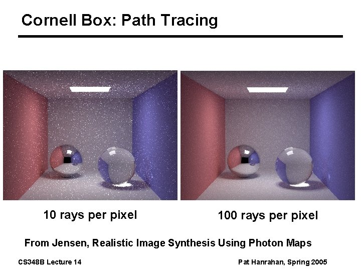
Cornell Box: Path Tracing 10 rays per pixel 100 rays per pixel From Jensen, Realistic Image Synthesis Using Photon Maps CS 348 B Lecture 14 Pat Hanrahan, Spring 2005

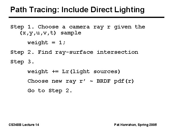
Path Tracing: Include Direct Lighting Step 1. Choose a camera ray r given the (x, y, u, v, t) sample weight = 1; Step 2. Find ray-surface intersection Step 3. weight += Lr(light sources) Choose new ray r’ ~ BRDF pdf(r) Go to Step 2. CS 348 B Lecture 14 Pat Hanrahan, Spring 2005

Discrete Random Walk

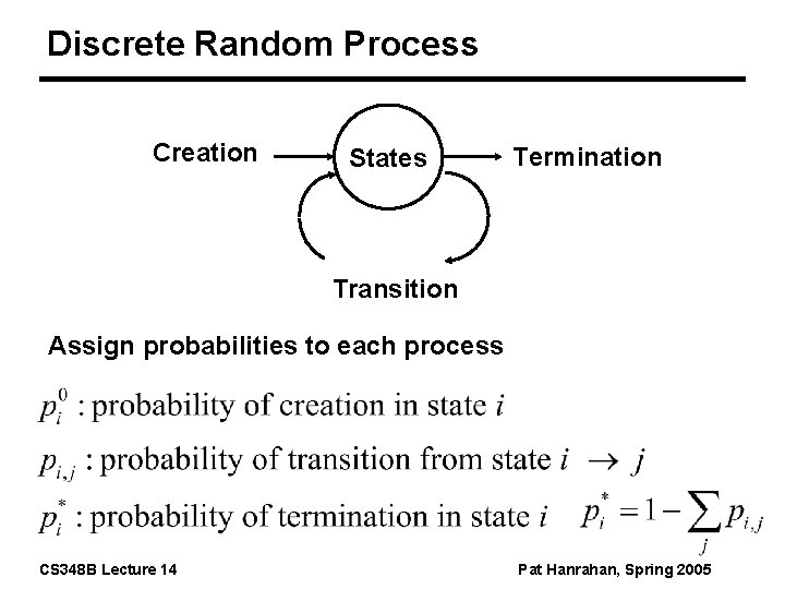
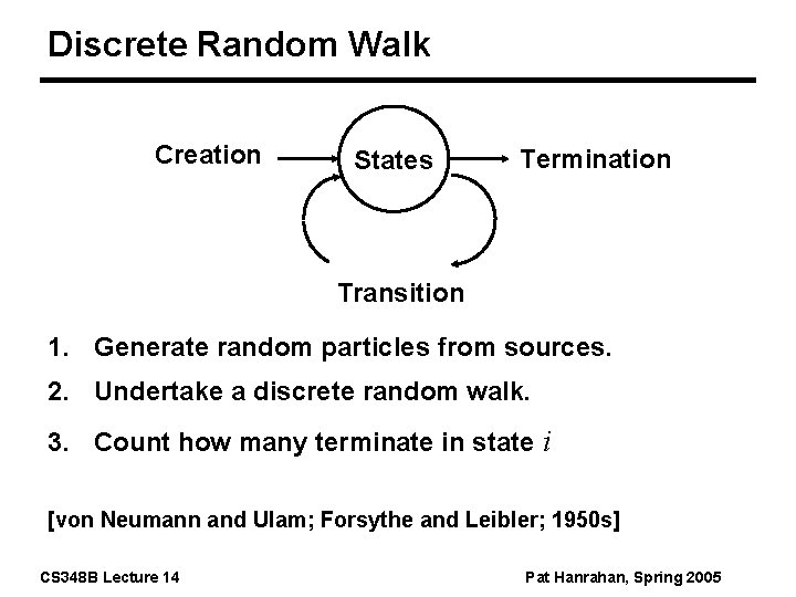
Discrete Random Process Creation States Termination Transition Assign probabilities to each process CS 348 B Lecture 14 Pat Hanrahan, Spring 2005

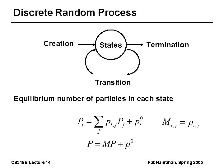
Discrete Random Process Creation States Termination Transition Equilibrium number of particles in each state CS 348 B Lecture 14 Pat Hanrahan, Spring 2005

Discrete Random Walk Creation States Termination Transition 1. Generate random particles from sources. 2. Undertake a discrete random walk. 3. Count how many terminate in state i [von Neumann and Ulam; Forsythe and Leibler; 1950 s] CS 348 B Lecture 14 Pat Hanrahan, Spring 2005

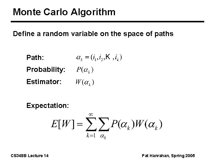
Monte Carlo Algorithm Define a random variable on the space of paths Path: Probability: Estimator: Expectation: CS 348 B Lecture 14 Pat Hanrahan, Spring 2005

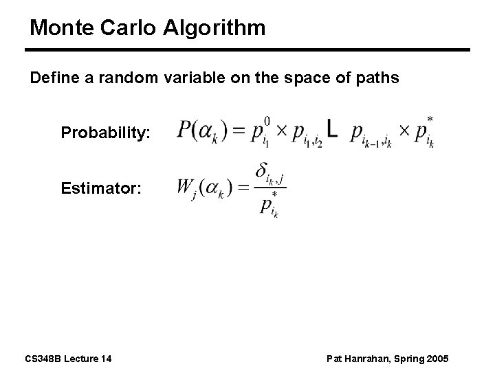
Monte Carlo Algorithm Define a random variable on the space of paths Probability: Estimator: CS 348 B Lecture 14 Pat Hanrahan, Spring 2005

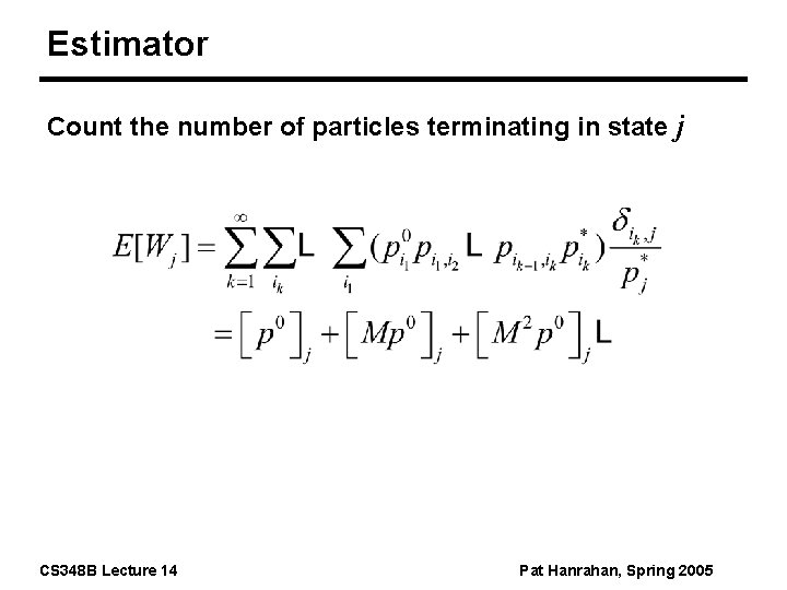
Estimator Count the number of particles terminating in state j CS 348 B Lecture 14 Pat Hanrahan, Spring 2005

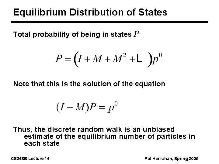
Equilibrium Distribution of States Total probability of being in states P Note that this is the solution of the equation Thus, the discrete random walk is an unbiased estimate of the equilibrium number of particles in each state CS 348 B Lecture 14 Pat Hanrahan, Spring 2005

Light Ray Tracing

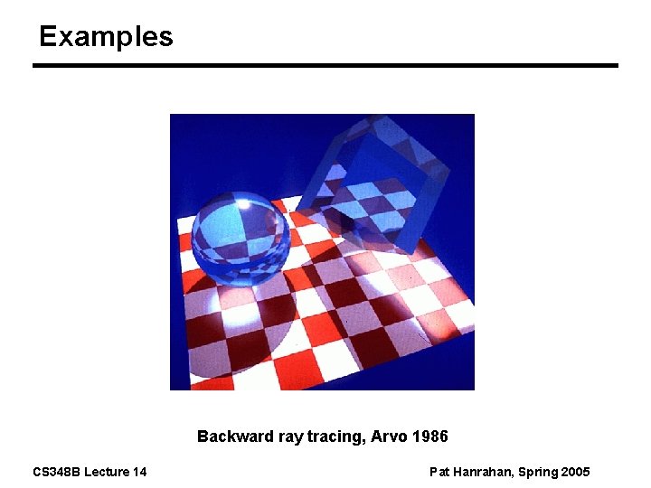
Examples Backward ray tracing, Arvo 1986 CS 348 B Lecture 14 Pat Hanrahan, Spring 2005

Path Tracing: From Lights Step 1. Choose a light ray Choose a light source according to the light source power distribution function. Choose a ray from the light source radiance (area) or intensity (point) distribution function w = 1; Step 2. Trace ray to find surface intersect Step 3. Interaction CS 348 B Lecture 14 Pat Hanrahan, Spring 2005

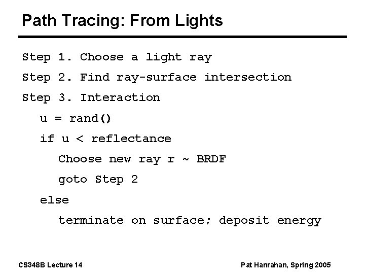
Path Tracing: From Lights Step 1. Choose a light ray Step 2. Find ray-surface intersection Step 3. Interaction u = rand() if u < reflectance Choose new ray r ~ BRDF goto Step 2 else terminate on surface; deposit energy CS 348 B Lecture 14 Pat Hanrahan, Spring 2005

Bidirectional Path Tracing

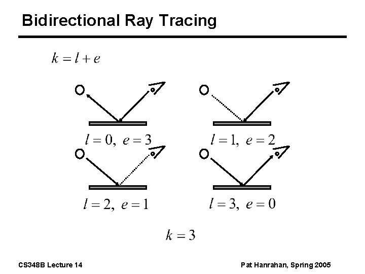
Bidirectional Ray Tracing CS 348 B Lecture 14 Pat Hanrahan, Spring 2005

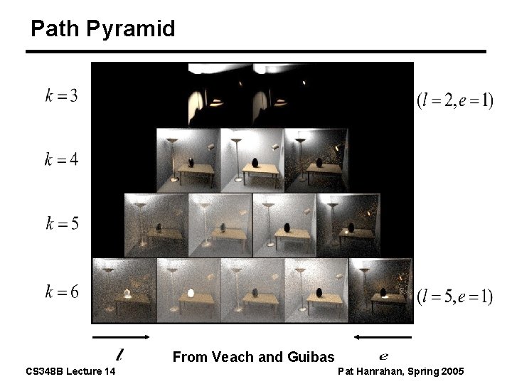
Path Pyramid From Veach and Guibas CS 348 B Lecture 14 Pat Hanrahan, Spring 2005

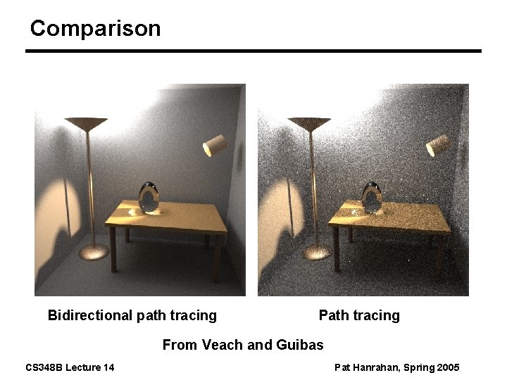
Comparison Bidirectional path tracing Path tracing From Veach and Guibas CS 348 B Lecture 14 Pat Hanrahan, Spring 2005

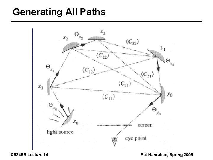
Generating All Paths CS 348 B Lecture 14 Pat Hanrahan, Spring 2005

Adjoint Formulation

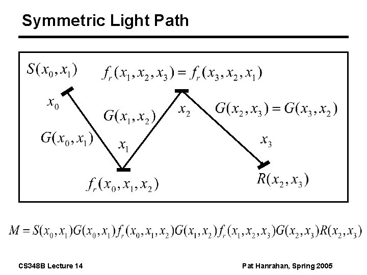
Symmetric Light Path CS 348 B Lecture 14 Pat Hanrahan, Spring 2005

Symmetric Light Path CS 348 B Lecture 14 Pat Hanrahan, Spring 2005

Symmetric Light Path CS 348 B Lecture 14 Pat Hanrahan, Spring 2005

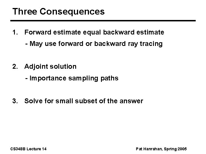
Three Consequences 1. Forward estimate equal backward estimate - May use forward or backward ray tracing 2. Adjoint solution - Importance sampling paths 3. Solve for small subset of the answer CS 348 B Lecture 14 Pat Hanrahan, Spring 2005

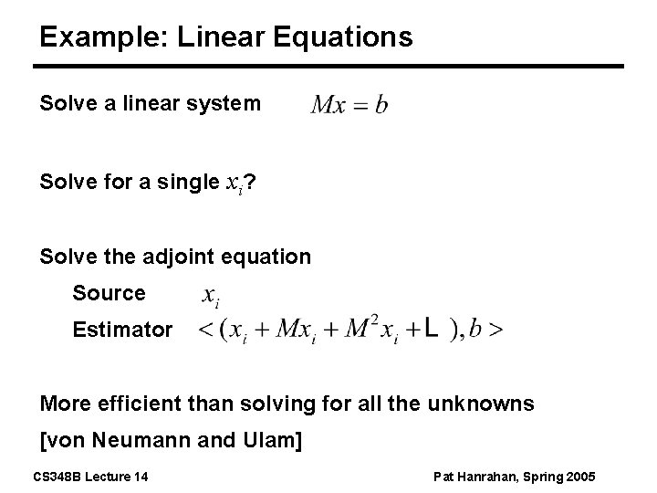
Example: Linear Equations Solve a linear system Solve for a single xi? Solve the adjoint equation Source Estimator More efficient than solving for all the unknowns [von Neumann and Ulam] CS 348 B Lecture 14 Pat Hanrahan, Spring 2005