Radiative Transfer Volume Path Tracing CS 295 Spring

Radiative Transfer & Volume Path Tracing CS 295, Spring 2017 Shuang Zhao Computer Science Department University of California, Irvine Modified from the original slides CS 295, Spring 2017 Shuang Zhao 1

Today’s Lecture • Radiative transfer • The mathematical model to simulate light scattering in participating media (e. g. , smoke) and translucent materials (e. g. , marble and skin) • Volume path tracing (VPT) • A Monte Carlo solution to the radiative transfer problem • Similar to the normal PT from previous lectures CS 295, Spring 2017 Shuang Zhao 2

Radiative Transfer CS 295: Realistic Image Synthesis CS 295, Spring 2017 Shuang Zhao 3

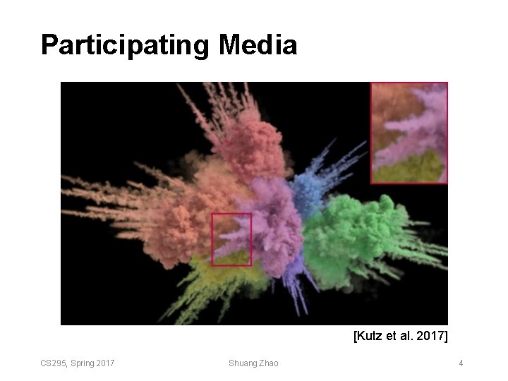
Participating Media [Kutz et al. 2017] CS 295, Spring 2017 Shuang Zhao 4

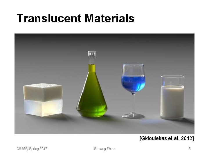
Translucent Materials [Gkioulekas et al. 2013] CS 295, Spring 2017 Shuang Zhao 5

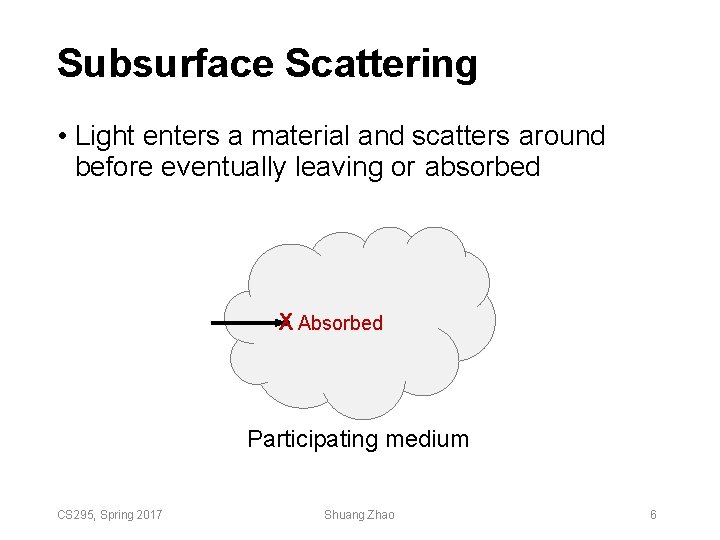
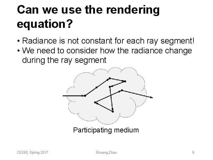
Subsurface Scattering • Light enters a material and scatters around before eventually leaving or absorbed X Absorbed Participating medium CS 295, Spring 2017 Shuang Zhao 6

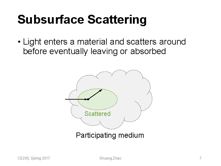
Subsurface Scattering • Light enters a material and scatters around before eventually leaving or absorbed Scattered Participating medium CS 295, Spring 2017 Shuang Zhao 7

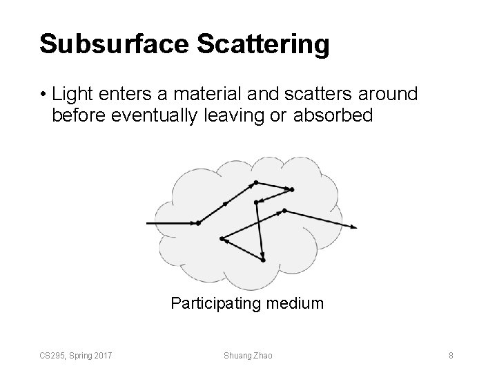
Subsurface Scattering • Light enters a material and scatters around before eventually leaving or absorbed Participating medium CS 295, Spring 2017 Shuang Zhao 8

Can we use the rendering equation? • Radiance is not constant for each ray segment! • We need to consider how the radiance change during the ray segment Participating medium CS 295, Spring 2017 Shuang Zhao 9

Radiative Transfer • A mathematical model describing how light interacts with participating media • Originated in physics • Now used in many areas • • • Astrophysics (light transport in space) Biomedicine (light transport in human tissue) Graphics Nuclear science & engineering (neutron transport) Remote sensing … CS 295, Spring 2017 Shuang Zhao 10

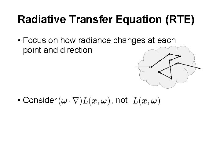
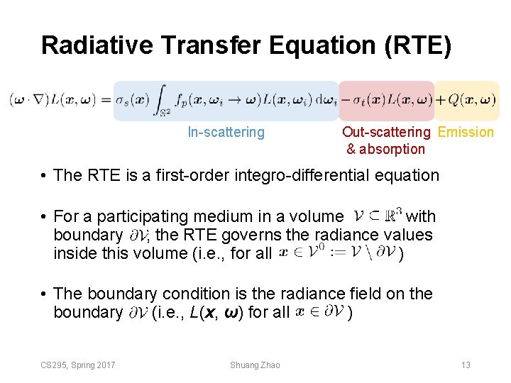
Radiative Transfer Equation (RTE) • Focus on how radiance changes at each point and direction • Consider , not

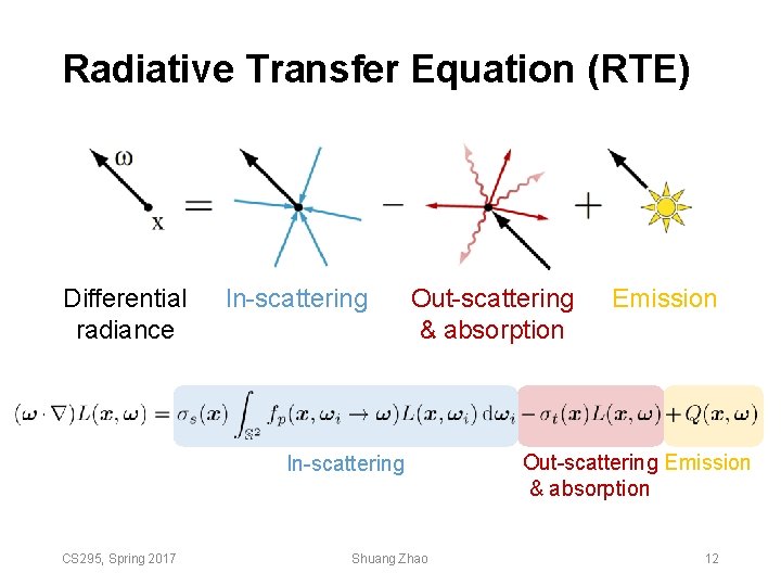
Radiative Transfer Equation (RTE) Differential radiance In-scattering Out-scattering & absorption In-scattering CS 295, Spring 2017 Shuang Zhao Emission Out-scattering Emission & absorption 12

Radiative Transfer Equation (RTE) In-scattering Out-scattering Emission & absorption • The RTE is a first-order integro-differential equation • For a participating medium in a volume with boundary , the RTE governs the radiance values inside this volume (i. e. , for all ) • The boundary condition is the radiance field on the boundary (i. e. , L(x, ω) for all ) CS 295, Spring 2017 Shuang Zhao 13

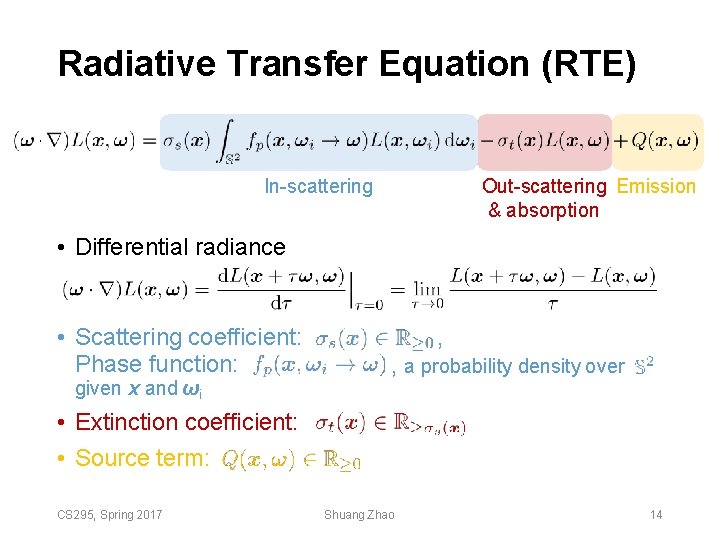
Radiative Transfer Equation (RTE) Out-scattering Emission & absorption In-scattering • Differential radiance • Scattering coefficient: Phase function: given x and ωi , , a probability density over • Extinction coefficient: • Source term: CS 295, Spring 2017 Shuang Zhao 14

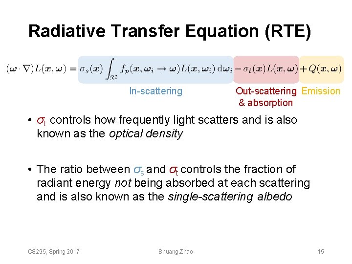
Radiative Transfer Equation (RTE) In-scattering Out-scattering Emission & absorption • σt controls how frequently light scatters and is also known as the optical density • The ratio between σs and σt controls the fraction of radiant energy not being absorbed at each scattering and is also known as the single-scattering albedo CS 295, Spring 2017 Shuang Zhao 15

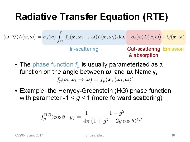
Radiative Transfer Equation (RTE) In-scattering Out-scattering Emission & absorption • The phase function fp is usually parameterized as a function on the angle between ωi and ω. Namely, • Example: the Henyey-Greenstein (HG) phase function with parameter -1 < g < 1 (more forward scattering): CS 295, Spring 2017 Shuang Zhao 16

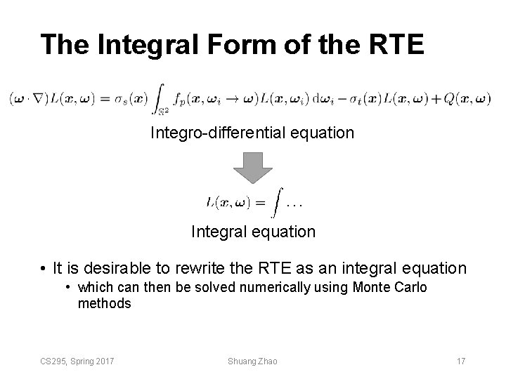
The Integral Form of the RTE Integro-differential equation Integral equation • It is desirable to rewrite the RTE as an integral equation • which can then be solved numerically using Monte Carlo methods CS 295, Spring 2017 Shuang Zhao 17

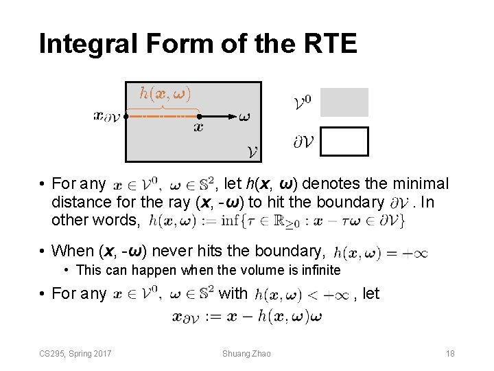
Integral Form of the RTE • For any , let h(x, ω) denotes the minimal distance for the ray (x, -ω) to hit the boundary. In other words, • When (x, -ω) never hits the boundary, • This can happen when the volume is infinite • For any CS 295, Spring 2017 with Shuang Zhao , let 18

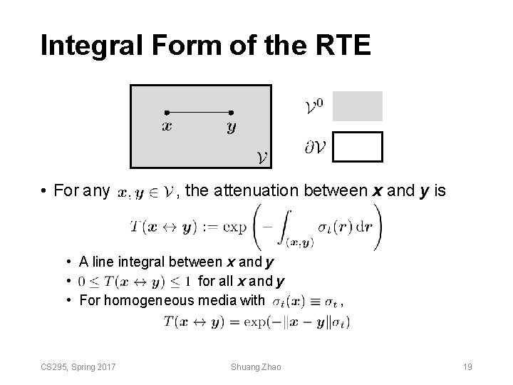
Integral Form of the RTE • For any , the attenuation between x and y is • A line integral between x and y • for all x and y • For homogeneous media with CS 295, Spring 2017 Shuang Zhao , 19

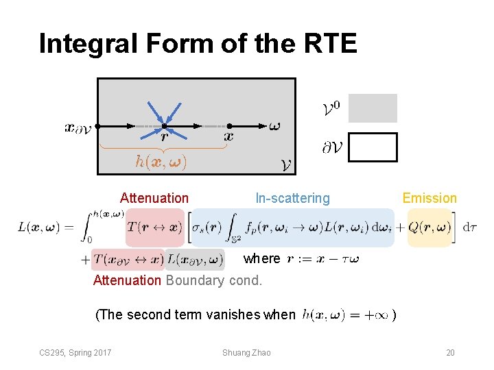
Integral Form of the RTE Attenuation In-scattering Emission where Attenuation Boundary cond. (The second term vanishes when CS 295, Spring 2017 Shuang Zhao ) 20

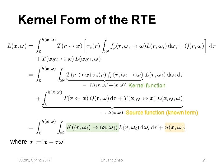
Kernel Form of the RTE Kernel function Source function (known term) where CS 295, Spring 2017 Shuang Zhao 21

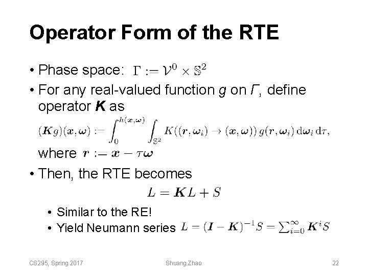
Operator Form of the RTE • Phase space: • For any real-valued function g on Γ, define operator K as where • Then, the RTE becomes • Similar to the RE! • Yield Neumann series CS 295, Spring 2017 Shuang Zhao 22

Start from here… Volume Path Tracing CS 295: Realistic Image Synthesis CS 295, Spring 2017 Shuang Zhao 23

Solving the RTE • Given the similarity between the RTE and the RE, Monte Carlo solutions to the RE can be adapted to solve the RTE • • Volume path tracing Volume adjoint particle tracing Volume bidirectional path tracing … CS 295, Spring 2017 Shuang Zhao 24

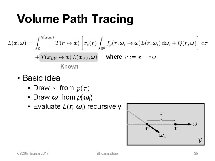
Volume Path Tracing where Known • Basic idea • Draw from • Draw ωi from p(ωi) • Evaluate L(r, ωi) recursively CS 295, Spring 2017 Shuang Zhao 25

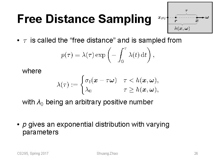
Free Distance Sampling • is called the “free distance” and is sampled from where with λ 0 being an arbitrary positive number • p gives an exponential distribution with varying parameters CS 295, Spring 2017 Shuang Zhao 26

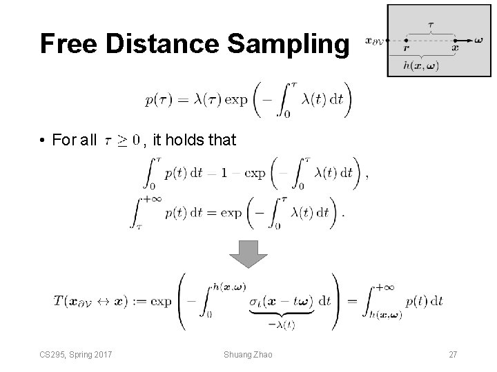
Free Distance Sampling • For all CS 295, Spring 2017 , it holds that Shuang Zhao 27

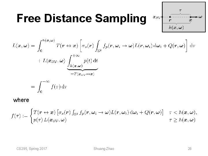
Free Distance Sampling where CS 295, Spring 2017 Shuang Zhao 28

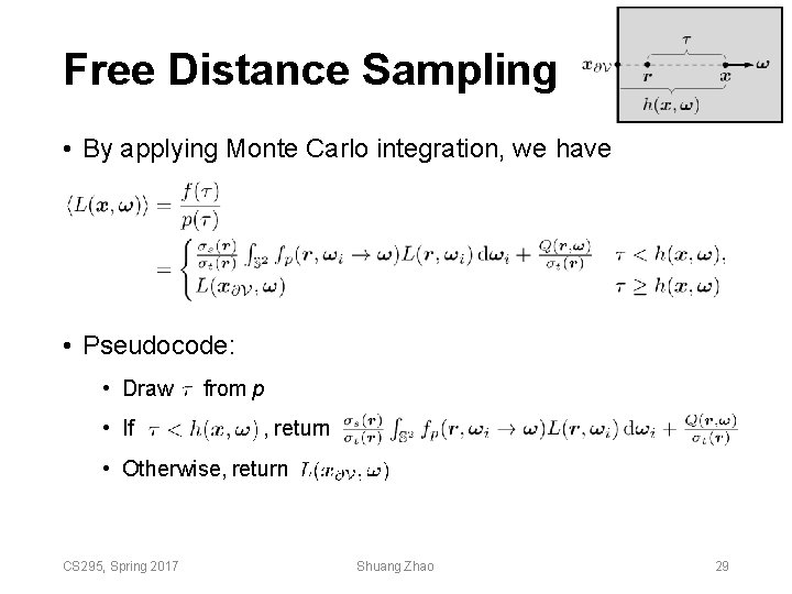
Free Distance Sampling • By applying Monte Carlo integration, we have • Pseudocode: • Draw • If from p , return • Otherwise, return CS 295, Spring 2017 Shuang Zhao 29

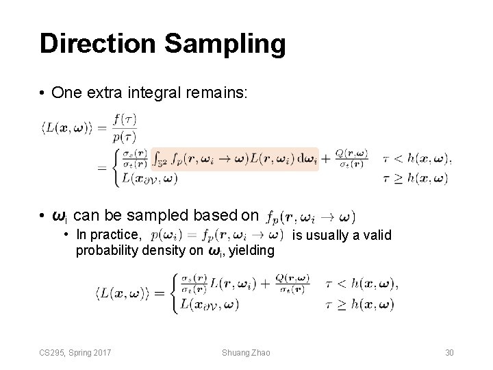
Direction Sampling • One extra integral remains: • ωi can be sampled based on • In practice, probability density on ωi, yielding CS 295, Spring 2017 Shuang Zhao is usually a valid 30

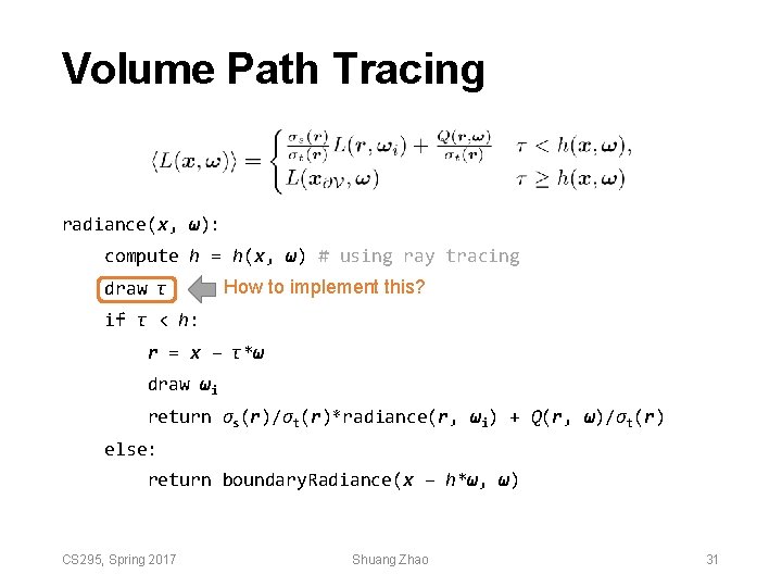
Volume Path Tracing radiance(x, ω): compute h = h(x, ω) # using ray tracing draw τ How to implement this? if τ < h: r = x – τ*ω draw ωi return σs(r)/σt(r)*radiance(r, ωi) + Q(r, ω)/σt(r) else: return boundary. Radiance(x – h*ω, ω) CS 295, Spring 2017 Shuang Zhao 31

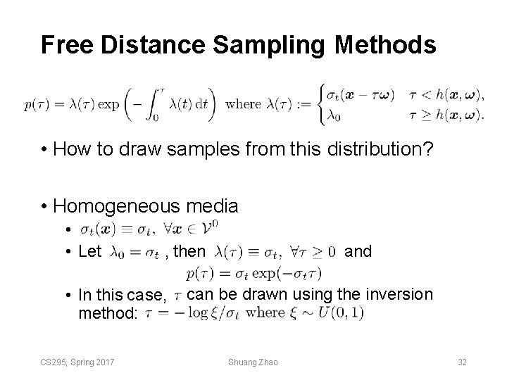
Free Distance Sampling Methods • How to draw samples from this distribution? • Homogeneous media • • Let , then • In this case, method: CS 295, Spring 2017 and can be drawn using the inversion Shuang Zhao 32

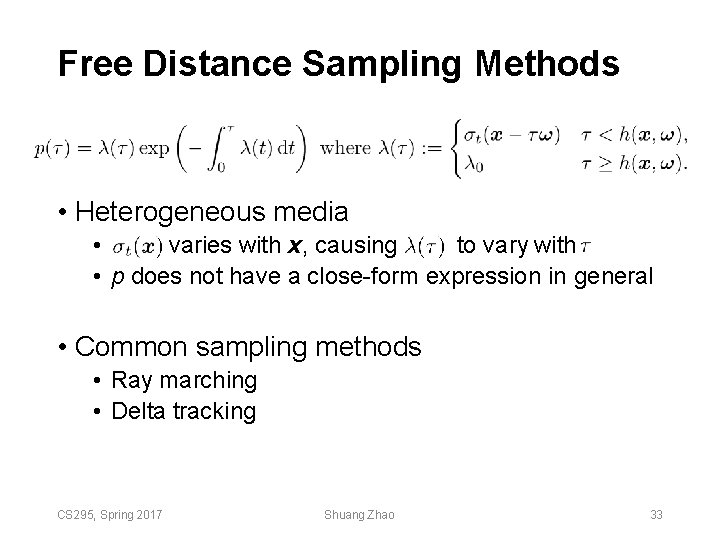
Free Distance Sampling Methods • Heterogeneous media • varies with x, causing to vary with • p does not have a close-form expression in general • Common sampling methods • Ray marching • Delta tracking CS 295, Spring 2017 Shuang Zhao 33

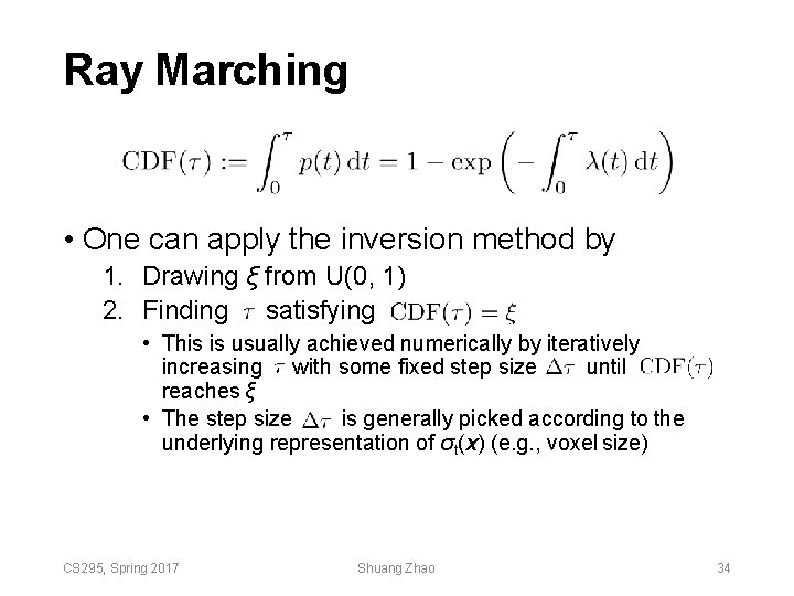
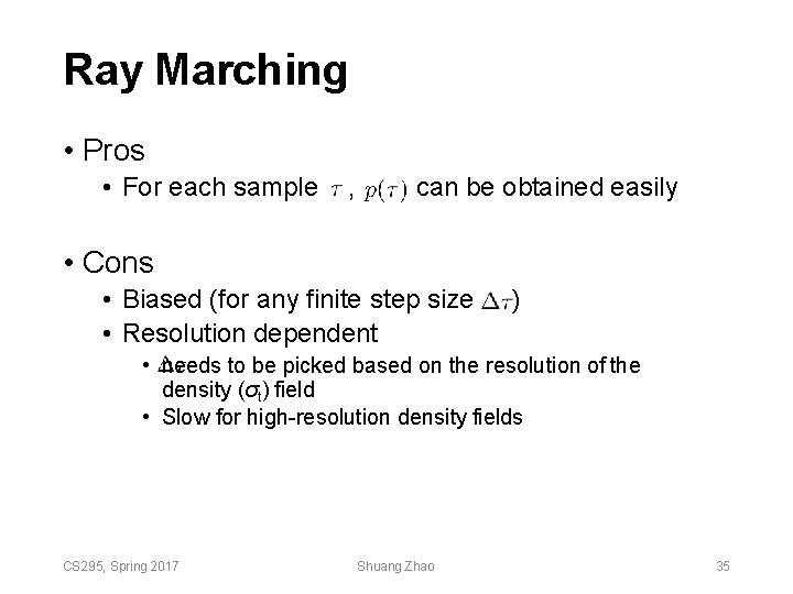
Ray Marching • One can apply the inversion method by 1. Drawing ξ from U(0, 1) 2. Finding satisfying • This is usually achieved numerically by iteratively increasing with some fixed step size until reaches ξ • The step size is generally picked according to the underlying representation of σt(x) (e. g. , voxel size) CS 295, Spring 2017 Shuang Zhao 34

Ray Marching • Pros • For each sample , can be obtained easily • Cons • Biased (for any finite step size • Resolution dependent ) • needs to be picked based on the resolution of the density (σt) field • Slow for high-resolution density fields CS 295, Spring 2017 Shuang Zhao 35

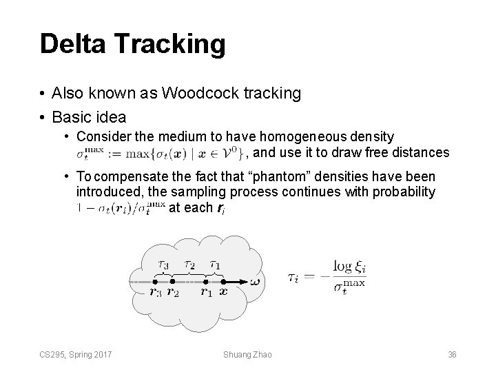
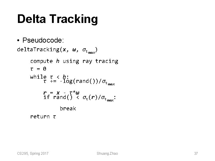
Delta Tracking • Also known as Woodcock tracking • Basic idea • Consider the medium to have homogeneous density , and use it to draw free distances • To compensate the fact that “phantom” densities have been introduced, the sampling process continues with probability at each ri CS 295, Spring 2017 Shuang Zhao 36

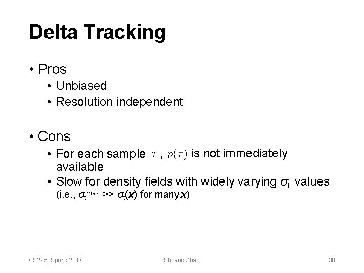
Delta Tracking • Pseudocode: delta. Tracking(x, ω, σt max) compute h using ray tracing τ = 0 while τ < h: τ += -log(rand())/σt max r = x - τ*ω if rand() < σt(r)/σt max: break return τ CS 295, Spring 2017 Shuang Zhao 37

Delta Tracking • Pros • Unbiased • Resolution independent • Cons is not immediately • For each sample , available • Slow for density fields with widely varying σt values (i. e. , σtmax >> σt(x) for many x) CS 295, Spring 2017 Shuang Zhao 38

Volume Path Tracing (VPT) radiance(x, ω): compute h = h(x, ω) draw τ if τ < h: r = x – τ*ω This basic version can be improved using techniques we have seen earlier: • Russian roulette • Next-event estimation • Multiple importance sampling draw ωi return σs(r)/σt(r)*radiance(r, ωi) + Q(r, ω)/σt(r) else: return boundary. Radiance(x – h*ω, ω) CS 295, Spring 2017 Shuang Zhao 39

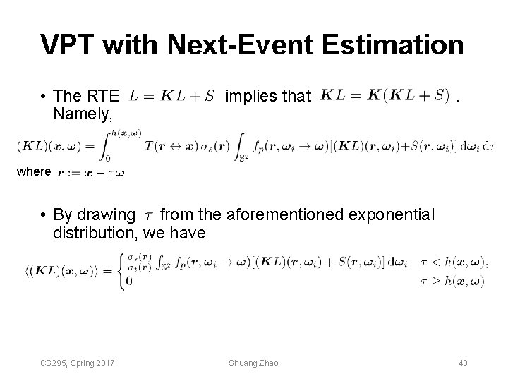
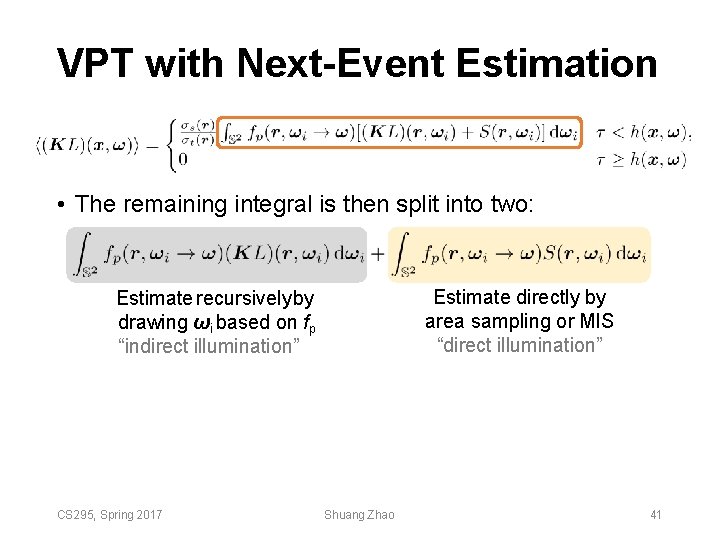
VPT with Next-Event Estimation • The RTE Namely, implies that . where • By drawing from the aforementioned exponential distribution, we have CS 295, Spring 2017 Shuang Zhao 40

VPT with Next-Event Estimation • The remaining integral is then split into two: Estimate directly by area sampling or MIS “direct illumination” Estimate recursively by drawing ωi based on fp “indirect illumination” CS 295, Spring 2017 Shuang Zhao 41

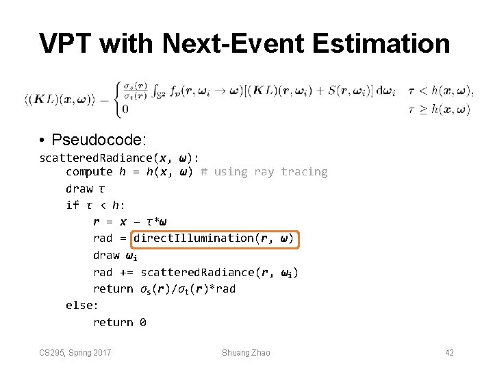
VPT with Next-Event Estimation • Pseudocode: scattered. Radiance(x, ω): compute h = h(x, ω) # using ray tracing draw τ if τ < h: r = x – τ*ω rad = direct. Illumination(r, ω) draw ωi rad += scattered. Radiance(r, ωi) return σs(r)/σt(r)*rad else: return 0 CS 295, Spring 2017 Shuang Zhao 42

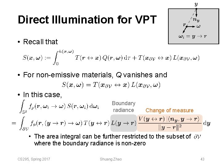
Direct Illumination for VPT • Recall that • For non-emissive materials, Q vanishes and • In this case, Boundary radiance Change of measure • The area integral can be further restricted to the subset of where the boundary radiance is non-zero CS 295, Spring 2017 Shuang Zhao 43

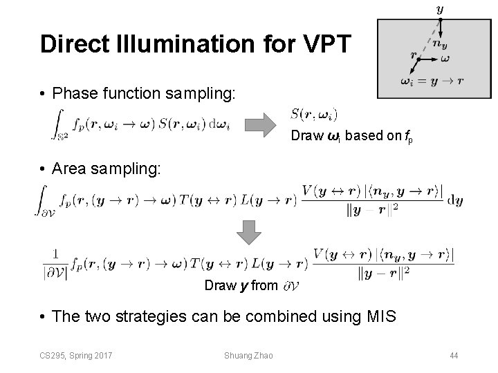
Direct Illumination for VPT • Phase function sampling: Draw ωi based on fp • Area sampling: Draw y from • The two strategies can be combined using MIS CS 295, Spring 2017 Shuang Zhao 44