CS 60050 Machine Learning 17 Jan 2008 CS

CS 60050 Machine Learning 17 Jan 2008

CS 391 L: Machine Learning: Decision Tree Learning Raymond J. Mooney University of Texas at Austin

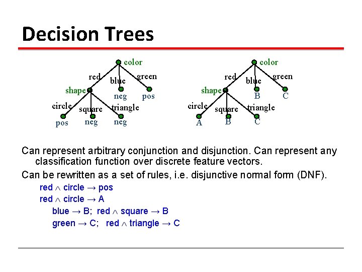
Decision Trees color red shape blue color green pos neg circle square triangle neg pos red shape blue green C B circle square triangle B C A Can represent arbitrary conjunction and disjunction. Can represent any classification function over discrete feature vectors. Can be rewritten as a set of rules, i. e. disjunctive normal form (DNF). red circle → pos red circle → A blue → B; red square → B green → C; red triangle → C

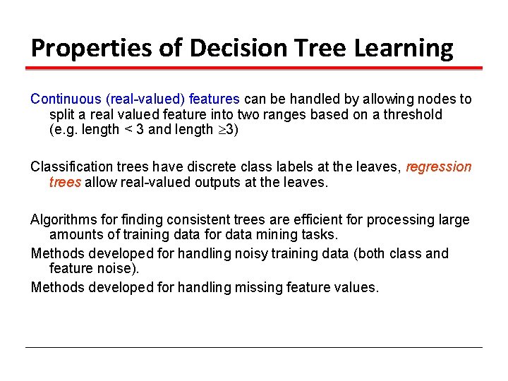
Properties of Decision Tree Learning Continuous (real-valued) features can be handled by allowing nodes to split a real valued feature into two ranges based on a threshold (e. g. length < 3 and length 3) Classification trees have discrete class labels at the leaves, regression trees allow real-valued outputs at the leaves. Algorithms for finding consistent trees are efficient for processing large amounts of training data for data mining tasks. Methods developed for handling noisy training data (both class and feature noise). Methods developed for handling missing feature values.

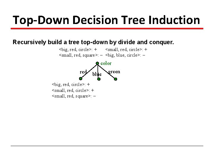
Top-Down Decision Tree Induction Recursively build a tree top-down by divide and conquer. <big, red, circle>: + <small, red, square>: <big, blue, circle>: color red blue <big, red, circle>: + <small, red, square>: green

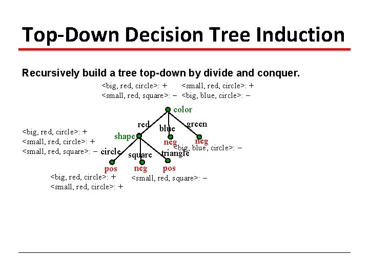
Top-Down Decision Tree Induction Recursively build a tree top-down by divide and conquer. <big, red, circle>: + <small, red, square>: <big, blue, circle>: color green blue <big, red, circle>: + shape neg <small, red, circle>: + neg <big, blue, circle>: <small, red, square>: circle square triangle pos neg pos red <big, red, circle>: + <small, red, square>:

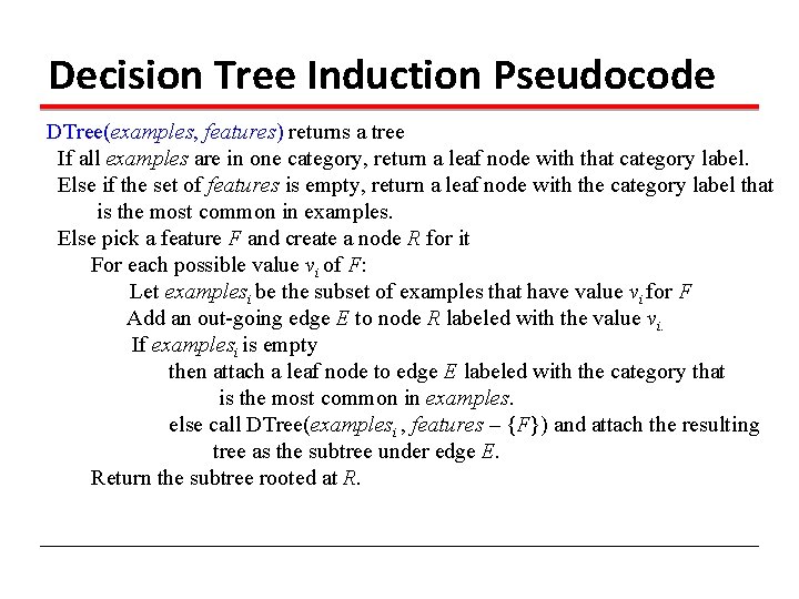
Decision Tree Induction Pseudocode DTree(examples, features) returns a tree If all examples are in one category, return a leaf node with that category label. Else if the set of features is empty, return a leaf node with the category label that is the most common in examples. Else pick a feature F and create a node R for it For each possible value vi of F: Let examplesi be the subset of examples that have value vi for F Add an out-going edge E to node R labeled with the value vi. If examplesi is empty then attach a leaf node to edge E labeled with the category that is the most common in examples. else call DTree(examplesi , features – {F}) and attach the resulting tree as the subtree under edge E. Return the subtree rooted at R.

Picking a Good Split Feature Goal is to have the resulting tree be as small as possible, per Occam’s razor. Finding a minimal decision tree (nodes, leaves, or depth) is an NP-hard optimization problem. Top-down divide-and-conquer method does a greedy search for a simple tree but does not guarantee to find the smallest. General lesson in ML: “Greed is good. ” Want to pick a feature that creates subsets of examples that are relatively “pure” in a single class so they are “closer” to being leaf nodes. There a variety of heuristics for picking a good test, a popular one is based on information gain that originated with the ID 3 system of Quinlan (1979).

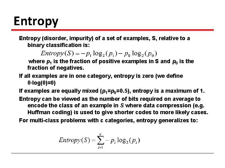
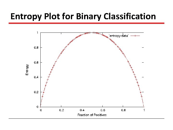
Entropy (disorder, impurity) of a set of examples, S, relative to a binary classification is: where p 1 is the fraction of positive examples in S and p 0 is the fraction of negatives. If all examples are in one category, entropy is zero (we define 0 log(0)=0) If examples are equally mixed (p 1=p 0=0. 5), entropy is a maximum of 1. Entropy can be viewed as the number of bits required on average to encode the class of an example in S where data compression (e. g. Huffman coding) is used to give shorter codes to more likely cases. For multi-class problems with c categories, entropy generalizes to:

Entropy Plot for Binary Classification

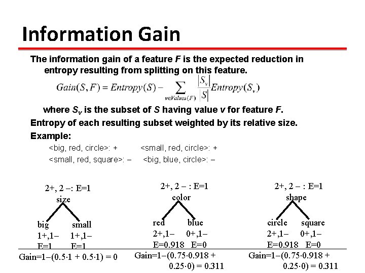
Information Gain The information gain of a feature F is the expected reduction in entropy resulting from splitting on this feature. where Sv is the subset of S having value v for feature F. Entropy of each resulting subset weighted by its relative size. Example: <big, red, circle>: + <small, red, square>: 2+, 2 : E=1 size big small 1+, 1 E=1 Gain=1 (0. 5 1 + 0. 5 1) = 0 <small, red, circle>: + <big, blue, circle>: 2+, 2 : E=1 color red blue 2+, 1 0+, 1 E=0. 918 E=0 Gain=1 (0. 75 0. 918 + 0. 25 0) = 0. 311 2+, 2 : E=1 shape circle square 2+, 1 0+, 1 E=0. 918 E=0 Gain=1 (0. 75 0. 918 + 0. 25 0) = 0. 311

Hypothesis Space Search Performs batch learning that processes all training instances at once rather than incremental learning that updates a hypothesis after each example. Performs hill-climbing (greedy search) that may only find a locally-optimal solution. Guaranteed to find a tree consistent with any conflict-free training set (i. e. identical feature vectors always assigned the same class), but not necessarily the simplest tree. Finds a single discrete hypothesis, so there is no way to provide confidences or create useful queries.

Bias in Decision-Tree Induction Information-gain gives a bias for trees with minimal depth. Implements a search (preference) bias instead of a language (restriction) bias.

History of Decision-Tree Research Hunt and colleagues use exhaustive search decision-tree methods (CLS) to model human concept learning in the 1960’s. In the late 70’s, Quinlan developed ID 3 with the information gain heuristic to learn expert systems from examples. Simulataneously, Breiman and Friedman and colleagues develop CART (Classification and Regression Trees), similar to ID 3. In the 1980’s a variety of improvements are introduced to handle noise, continuous features, missing features, and improved splitting criteria. Various expert-system development tools results. Quinlan’s updated decision-tree package (C 4. 5) released in 1993. Weka includes Java version of C 4. 5 called J 48.

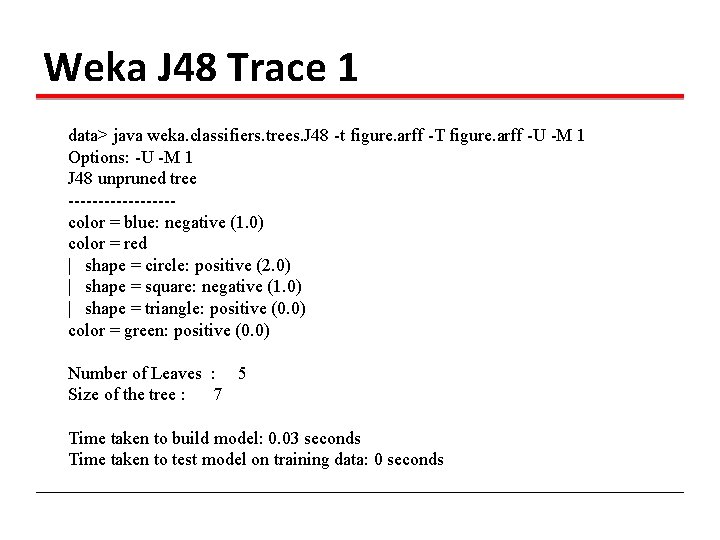
Weka J 48 Trace 1 data> java weka. classifiers. trees. J 48 -t figure. arff -T figure. arff -U -M 1 Options: -U -M 1 J 48 unpruned tree ---------color = blue: negative (1. 0) color = red | shape = circle: positive (2. 0) | shape = square: negative (1. 0) | shape = triangle: positive (0. 0) color = green: positive (0. 0) Number of Leaves : 5 Size of the tree : 7 Time taken to build model: 0. 03 seconds Time taken to test model on training data: 0 seconds

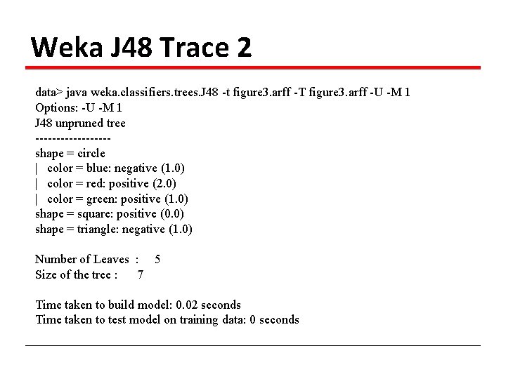
Weka J 48 Trace 2 data> java weka. classifiers. trees. J 48 -t figure 3. arff -T figure 3. arff -U -M 1 Options: -U -M 1 J 48 unpruned tree ---------shape = circle | color = blue: negative (1. 0) | color = red: positive (2. 0) | color = green: positive (1. 0) shape = square: positive (0. 0) shape = triangle: negative (1. 0) Number of Leaves : 5 Size of the tree : 7 Time taken to build model: 0. 02 seconds Time taken to test model on training data: 0 seconds

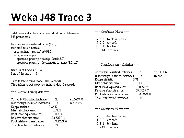
Weka J 48 Trace 3 data> java weka. classifiers. trees. J 48 -t contact-lenses. arff J 48 pruned tree ---------tear-prod-rate = reduced: none (12. 0) tear-prod-rate = normal | astigmatism = no: soft (6. 0/1. 0) | astigmatism = yes | | spectacle-prescrip = myope: hard (3. 0) | | spectacle-prescrip = hypermetrope: none (3. 0/1. 0) Number of Leaves : 4 Size of the tree : 7 Time taken to build model: 0. 03 seconds Time taken to test model on training data: 0 seconds === Error on training data === Correctly Classified Instances 22 91. 6667 % Incorrectly Classified Instances 2 8. 3333 % Kappa statistic 0. 8447 Mean absolute error 0. 0833 Root mean squared error 0. 2041 Relative absolute error 22. 6257 % Root relative squared error 48. 1223 % Total Number of Instances 24 === Confusion Matrix === a 5 0 1 b c <-- classified as 0 0 | a = soft 3 1 | b = hard 0 14 | c = none === Stratified cross-validation === Correctly Classified Instances 20 83. 3333 % Incorrectly Classified Instances 4 16. 6667 % Kappa statistic 0. 71 Mean absolute error 0. 15 Root mean squared error 0. 3249 Relative absolute error 39. 7059 % Root relative squared error 74. 3898 % Total Number of Instances 24 === Confusion Matrix === a 5 0 1 b c <-- classified as 0 0 | a = soft 3 1 | b = hard 2 12 | c = none

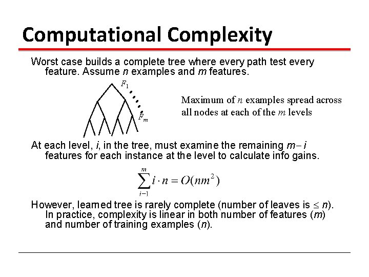
Computational Complexity Worst case builds a complete tree where every path test every feature. Assume n examples and m features. F 1 Fm Maximum of n examples spread across all nodes at each of the m levels At each level, i, in the tree, must examine the remaining m i features for each instance at the level to calculate info gains. However, learned tree is rarely complete (number of leaves is n). In practice, complexity is linear in both number of features (m) and number of training examples (n).

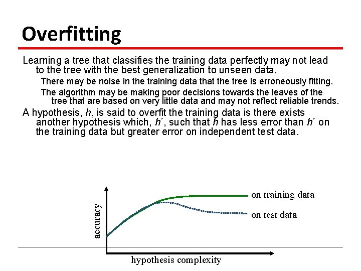
Overfitting Learning a tree that classifies the training data perfectly may not lead to the tree with the best generalization to unseen data. There may be noise in the training data that the tree is erroneously fitting. The algorithm may be making poor decisions towards the leaves of the tree that are based on very little data and may not reflect reliable trends. A hypothesis, h, is said to overfit the training data is there exists another hypothesis which, h´, such that h has less error than h´ on the training data but greater error on independent test data. accuracy on training data on test data hypothesis complexity

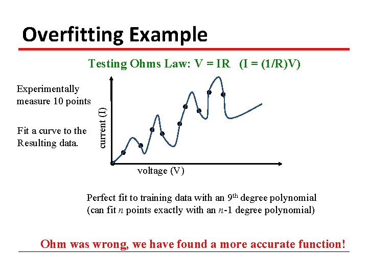
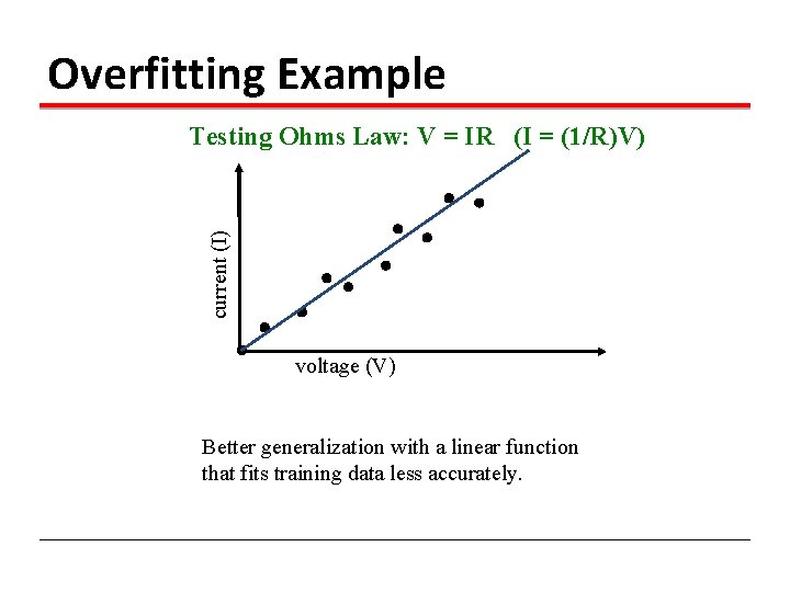
Overfitting Example Testing Ohms Law: V = IR (I = (1/R)V) Fit a curve to the Resulting data. current (I) Experimentally measure 10 points voltage (V) Perfect fit to training data with an 9 th degree polynomial (can fit n points exactly with an n-1 degree polynomial) Ohm was wrong, we have found a more accurate function!

Overfitting Example current (I) Testing Ohms Law: V = IR (I = (1/R)V) voltage (V) Better generalization with a linear function that fits training data less accurately.

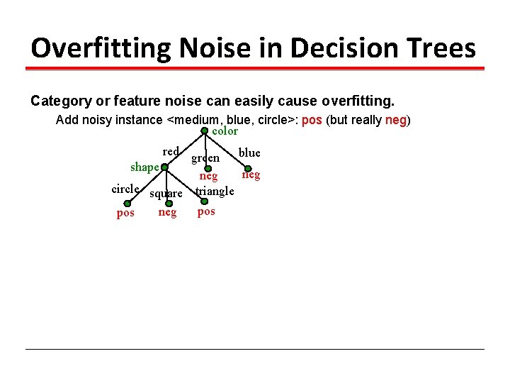
Overfitting Noise in Decision Trees Category or feature noise can easily cause overfitting. Add noisy instance <medium, blue, circle>: pos (but really neg) color red green blue shape neg circle square triangle pos neg pos

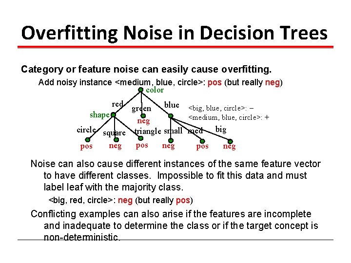
Overfitting Noise in Decision Trees Category or feature noise can easily cause overfitting. Add noisy instance <medium, blue, circle>: pos (but really neg) color red green blue <big, blue, circle>: shape <medium, blue, circle>: + neg circle square triangle small med big pos neg Noise can also cause different instances of the same feature vector to have different classes. Impossible to fit this data and must label leaf with the majority class. <big, red, circle>: neg (but really pos) Conflicting examples can also arise if the features are incomplete and inadequate to determine the class or if the target concept is non-deterministic.

Overfitting when our learning algorithm continues develop hypotheses that reduce training set error at the cost of an increased test set error. According to Mitchell, a hypothesis, h, is said to overfit the training set, D, when there exists a hypothesis, h’, that outperforms h on the total distribution of instances that D is a subset of. We can attempt to avoid overfitting by using a validation set. If we see that a subsequent tree reduces training set error but at the cost of an increased validation set error then we know we can stop growing the tree.

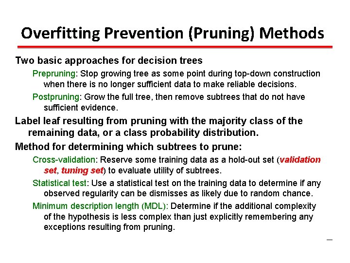
Overfitting Prevention (Pruning) Methods Two basic approaches for decision trees Prepruning: Stop growing tree as some point during top-down construction when there is no longer sufficient data to make reliable decisions. Postpruning: Grow the full tree, then remove subtrees that do not have sufficient evidence. Label leaf resulting from pruning with the majority class of the remaining data, or a class probability distribution. Method for determining which subtrees to prune: Cross-validation: Reserve some training data as a hold-out set (validation set, tuning set) to evaluate utility of subtrees. Statistical test: Use a statistical test on the training data to determine if any observed regularity can be dismisses as likely due to random chance. Minimum description length (MDL): Determine if the additional complexity of the hypothesis is less complex than just explicitly remembering any exceptions resulting from pruning.

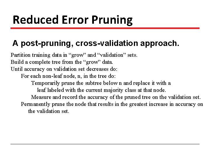
Reduced Error Pruning A post-pruning, cross-validation approach. Partition training data in “grow” and “validation” sets. Build a complete tree from the “grow” data. Until accuracy on validation set decreases do: For each non-leaf node, n, in the tree do: Temporarily prune the subtree below n and replace it with a leaf labeled with the current majority class at that node. Measure and record the accuracy of the pruned tree on the validation set. Permanently prune the node that results in the greatest increase in accuracy on the validation set.

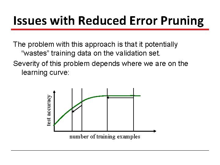
Issues with Reduced Error Pruning test accuracy The problem with this approach is that it potentially “wastes” training data on the validation set. Severity of this problem depends where we are on the learning curve: number of training examples

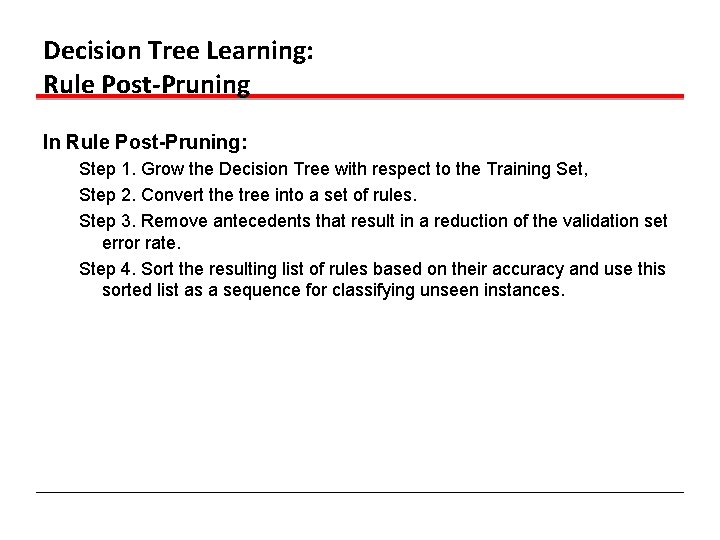
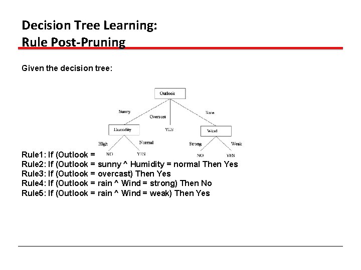
Decision Tree Learning: Rule Post-Pruning In Rule Post-Pruning: Step 1. Grow the Decision Tree with respect to the Training Set, Step 2. Convert the tree into a set of rules. Step 3. Remove antecedents that result in a reduction of the validation set error rate. Step 4. Sort the resulting list of rules based on their accuracy and use this sorted list as a sequence for classifying unseen instances.

Decision Tree Learning: Rule Post-Pruning Given the decision tree: Rule 1: If (Outlook = sunny ^ Humidity = high ) Then No Rule 2: If (Outlook = sunny ^ Humidity = normal Then Yes Rule 3: If (Outlook = overcast) Then Yes Rule 4: If (Outlook = rain ^ Wind = strong) Then No Rule 5: If (Outlook = rain ^ Wind = weak) Then Yes

Decision Tree Learning: Other Methods for Attribute Selection The information gain equation, G(S, A), presented earlier is biased toward attributes that have a large number of values over attributes that have a smaller number of values. The ‘Super Attributes’ will easily be selected as the root, result in a broad tree that classifies perfectly but performs poorly on unseen instances. We can penalize attributes with large numbers of values by using an alternative method for attribute selection, referred to as Gain. Ratio.

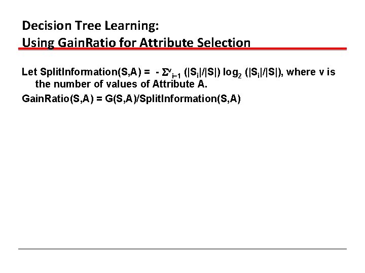
Decision Tree Learning: Using Gain. Ratio for Attribute Selection Let Split. Information(S, A) = - vi=1 (|Si|/|S|) log 2 (|Si|/|S|), where v is the number of values of Attribute A. Gain. Ratio(S, A) = G(S, A)/Split. Information(S, A)

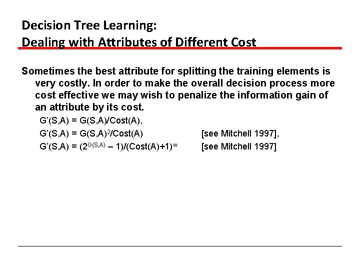
Decision Tree Learning: Dealing with Attributes of Different Cost Sometimes the best attribute for splitting the training elements is very costly. In order to make the overall decision process more cost effective we may wish to penalize the information gain of an attribute by its cost. G’(S, A) = G(S, A)/Cost(A), G’(S, A) = G(S, A)2/Cost(A) G’(S, A) = (2 G(S, A) – 1)/(Cost(A)+1)w [see Mitchell 1997], [see Mitchell 1997]

Cross-Validating without Losing Training Data If the algorithm is modified to grow trees breadth-first rather than depth-first, we can stop growing after reaching any specified tree complexity. First, run several trials of reduced error-pruning using different random splits of grow and validation sets. Record the complexity of the pruned tree learned in each trial. Let C be the average pruned-tree complexity. Grow a final tree breadth-first from all the training data but stop when the complexity reaches C. Similar cross-validation approach can be used to set arbitrary algorithm parameters in general.

Additional Decision Tree Issues Better splitting criteria Information gain prefers features with many values. Continuous features Predicting a real-valued function (regression trees) Missing feature values Features with costs Misclassification costs Incremental learning ID 4 ID 5 Mining large databases that do not fit in main memory

CS 391 L: Machine Learning: Ensembles Raymond J. Mooney University of Texas at Austin

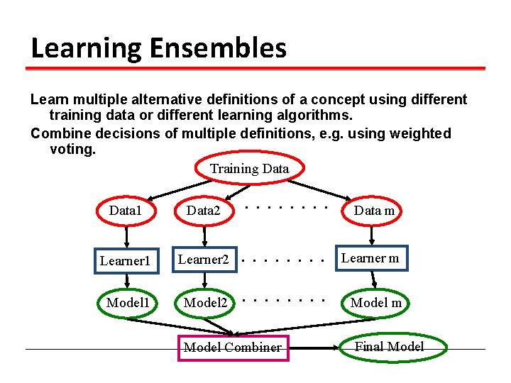
Learning Ensembles Learn multiple alternative definitions of a concept using different training data or different learning algorithms. Combine decisions of multiple definitions, e. g. using weighted voting. Training Data 1 Data 2 Data m Learner 1 Learner 2 Learner m Model 1 Model 2 Model m Model Combiner Final Model

Value of Ensembles When combing multiple independent and diverse decisions each of which is at least more accurate than random guessing, random errors cancel each other out, correct decisions are reinforced. Human ensembles are demonstrably better How many jelly beans in the jar? : Individual estimates vs. group average. Who Wants to be a Millionaire: Expert friend vs. audience vote.

Homogenous Ensembles Use a single, arbitrary learning algorithm but manipulate training data to make it learn multiple models. Data 1 Data 2 … Data m Learner 1 = Learner 2 = … = Learner m Different methods for changing training data: In Bagging: Resample training data Boosting: Reweight training data DECORATE: Add additional artificial training data WEKA, these are called meta-learners, they take a learning algorithm as an argument (base learner) and create a new learning algorithm.

Bagging Create ensembles by repeatedly randomly resampling the training data (Brieman, 1996). Given a training set of size n, create m samples of size n by drawing n examples from the original data, with replacement. Each bootstrap sample will on average contain 63. 2% of the unique training examples, the rest are replicates. Combine the m resulting models using simple majority vote. Decreases error by decreasing the variance in the results due to unstable learners, algorithms (like decision trees) whose output can change dramatically when the training data is slightly changed.

Boosting Originally developed by computational learning theorists to guarantee performance improvements on fitting training data for a weak learner that only needs to generate a hypothesis with a training accuracy greater than 0. 5 (Schapire, 1990). Revised to be a practical algorithm, Ada. Boost, for building ensembles that empirically improves generalization performance (Freund & Shapire, 1996). Examples are given weights. At each iteration, a new hypothesis is learned and the examples are reweighted to focus the system on examples that the most recently learned classifier got wrong.

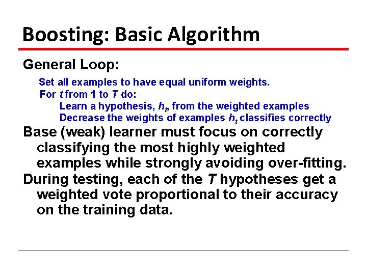
Boosting: Basic Algorithm General Loop: Set all examples to have equal uniform weights. For t from 1 to T do: Learn a hypothesis, ht, from the weighted examples Decrease the weights of examples ht classifies correctly Base (weak) learner must focus on correctly classifying the most highly weighted examples while strongly avoiding over-fitting. During testing, each of the T hypotheses get a weighted vote proportional to their accuracy on the training data.

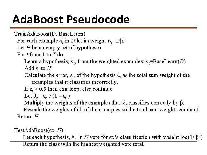
Ada. Boost Pseudocode Train. Ada. Boost(D, Base. Learn) For each example di in D let its weight wi=1/|D| Let H be an empty set of hypotheses For t from 1 to T do: Learn a hypothesis, ht, from the weighted examples: ht=Base. Learn(D) Add ht to H Calculate the error, εt, of the hypothesis ht as the total sum weight of the examples that it classifies incorrectly. If εt > 0. 5 then exit loop, else continue. Let βt = εt / (1 – εt ) Multiply the weights of the examples that ht classifies correctly by βt Rescale the weights of all of the examples so the total sum weight remains 1. Return H Test. Ada. Boost(ex, H) Let each hypothesis, ht, in H vote for ex’s classification with weight log(1/ βt ) Return the class with the highest weighted vote total.

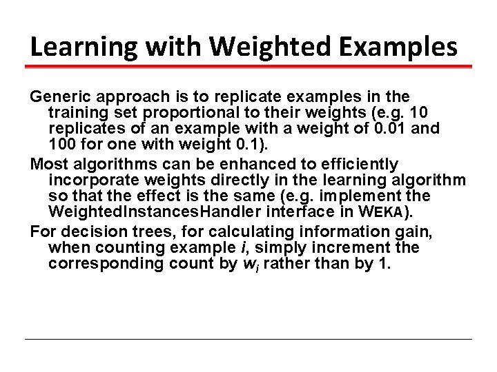
Learning with Weighted Examples Generic approach is to replicate examples in the training set proportional to their weights (e. g. 10 replicates of an example with a weight of 0. 01 and 100 for one with weight 0. 1). Most algorithms can be enhanced to efficiently incorporate weights directly in the learning algorithm so that the effect is the same (e. g. implement the Weighted. Instances. Handler interface in WEKA). For decision trees, for calculating information gain, when counting example i, simply increment the corresponding count by wi rather than by 1.

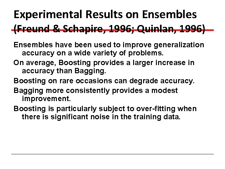
Experimental Results on Ensembles (Freund & Schapire, 1996; Quinlan, 1996) Ensembles have been used to improve generalization accuracy on a wide variety of problems. On average, Boosting provides a larger increase in accuracy than Bagging. Boosting on rare occasions can degrade accuracy. Bagging more consistently provides a modest improvement. Boosting is particularly subject to over-fitting when there is significant noise in the training data.

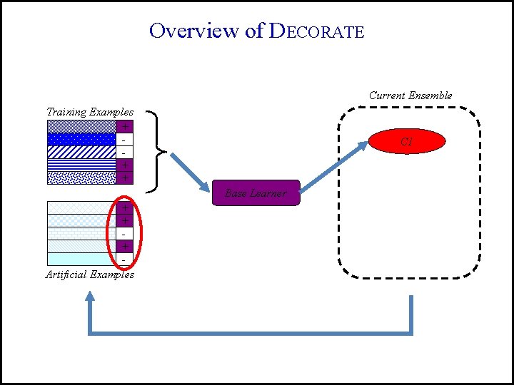
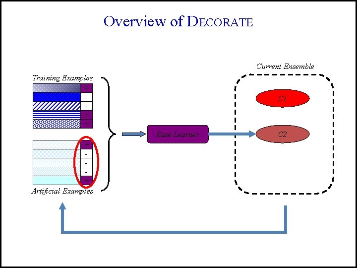
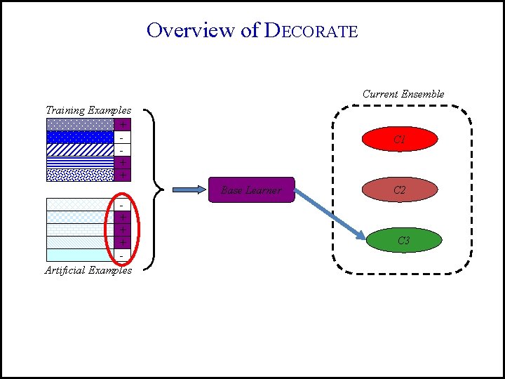
DECORATE (Melville & Mooney, 2003) Change training data by adding new artificial training examples that encourage diversity in the resulting ensemble. Improves accuracy when the training set is small, and therefore resampling and reweighting the training set has limited ability to generate diverse alternative hypotheses.

Overview of DECORATE Current Ensemble Training Examples + + + C 1 Base Learner + + + Artificial Examples

Overview of DECORATE Current Ensemble Training Examples + + + C 1 Base Learner + + + Artificial Examples C 2

Overview of DECORATE Current Ensemble Training Examples + + + C 1 Base Learner + + + Artificial Examples C 2 C 3

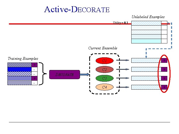
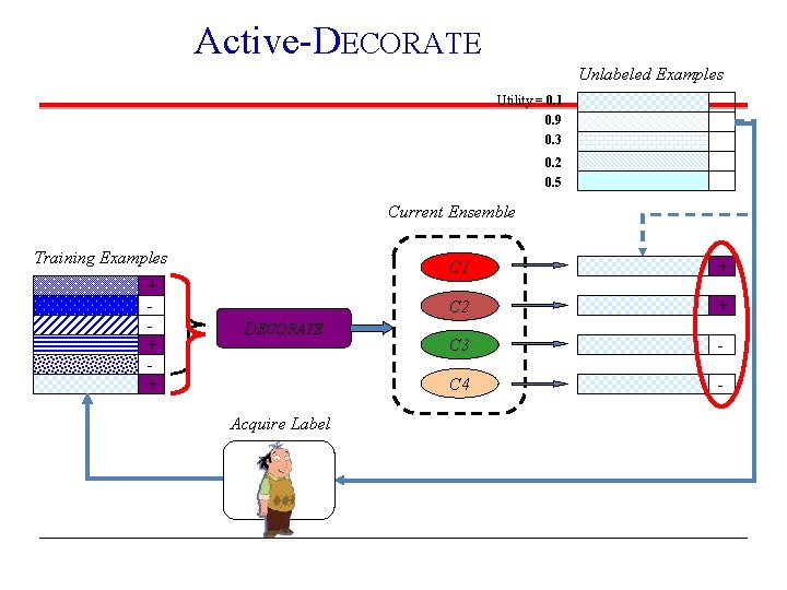
Ensembles and Active Learning Ensembles can be used to actively select good new training examples. Select the unlabeled example that causes the most disagreement amongst the members of the ensemble. Applicable to any ensemble method: Query. Bagging Query. Boosting Active. DECORATE

Active-DECORATE Unlabeled Examples Utility = 0. 1 Current Ensemble Training Examples + + - DECORATE C 1 + C 2 + C 3 + C 4 +

Active-DECORATE Unlabeled Examples Utility = 0. 1 0. 9 0. 3 0. 2 0. 5 Current Ensemble Training Examples + + + DECORATE Acquire Label C 1 + C 2 + C 3 - C 4 -

Issues in Ensembles Parallelism in Ensembles: Bagging is easily parallelized, Boosting is not. Variants of Boosting to handle noisy data. How “weak” should a base-learner for Boosting be? What is theoretical explanation of boosting’s ability to improve generalization? Exactly how does the diversity of ensembles affect their generalization performance. Combining Boosting and Bagging.