CS 347 Introduction to Artificial Intelligence CS 347

CS 347 – Introduction to Artificial Intelligence CS 347 course website: http: //web. mst. edu/~tauritzd/courses/cs 347/ Dr. Daniel Tauritz (Dr. T) Department of Computer Science tauritzd@mst. edu http: //web. mst. edu/~tauritzd/

What is AI? Systems that… –act like humans (Turing Test) –think like humans –think rationally –act rationally Play Ultimatum Game

Rational Agents • • • Environment Sensors (percepts) Actuators (actions) Agent Function Agent Program Performance Measures

Rational Behavior Depends on: • Agent’s performance measure • Agent’s prior knowledge • Possible percepts and actions • Agent’s percept sequence

Rational Agent Definition “For each possible percept sequence, a rational agent selects an action that is expected to maximize its performance measure, given the evidence provided by the percept sequence and any prior knowledge the agent has. ”

Task Environments PEAS description & properties: –Fully/Partially Observable –Deterministic, Stochastic, Strategic –Episodic, Sequential –Static, Dynamic, Semi-dynamic –Discrete, Continuous –Single agent, Multiagent –Competitive, Cooperative

Problem-solving agents A definition: Problem-solving agents are goal based agents that decide what to do based on an action sequence leading to a goal state.

Problem-solving steps • Problem-formulation (actions & states) • Goal-formulation (states) • Search (action sequences) • Execute solution

Well-defined problems • • • Initial state Action set Transition model: RESULT(s, a) Goal test Path cost Solution / optimal solution

Example problems • • Vacuum world Tic-tac-toe 8 -puzzle 8 -queens problem

Search trees • Root corresponds with initial state • Vacuum state space vs. search tree • Search algorithms iterate through goal testing and expanding a state until goal found • Order of state expansion is critical!

Search node datastructure • • n. STATE n. PARENT-NODE n. ACTION n. PATH-COST States are NOT search nodes!

Frontier • Frontier = Set of leaf nodes • Implemented as a queue with ops: – EMPTY? (queue) – POP(queue) – INSERT(element, queue) • Queue types: FIFO, LIFO (stack), and priority queue

Problem-solving performance • • Completeness Optimality Time complexity Space complexity

Complexity in AI • • b – branching factor d – depth of shallowest goal node m – max path length in state space Time complexity: # generated nodes Space complexity: max # nodes stored Search cost: time + space complexity Total cost: search + path cost

Tree Search • • • Breadth First Tree Search (BFTS) Uniform Cost Tree Search (UCTS) Depth-First Tree Search (DFTS) Depth-Limited Tree Search (DLTS) Iterative-Deepening Depth-First Tree Search (ID-DFTS)

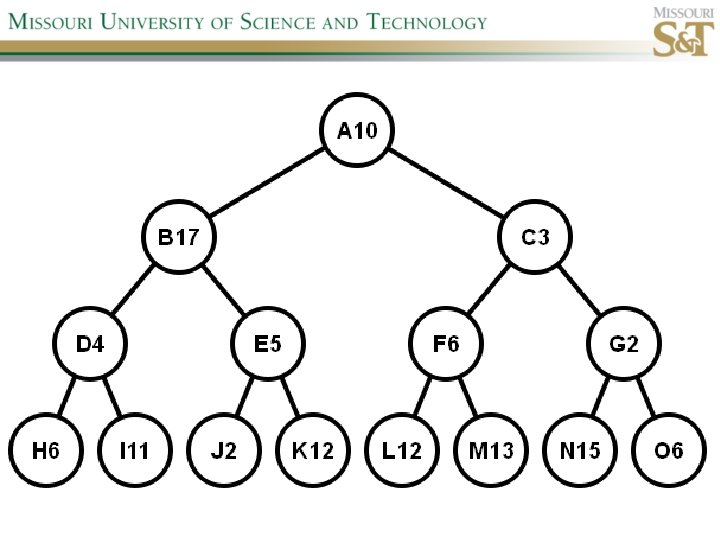
Example state space #1

Breadth First Tree Search (BFTS) • Frontier: FIFO queue • Complete: if b and d are finite • Optimal: if path-cost is non-decreasing function of depth • Time complexity: O(b^d) • Space complexity: O(b^d)

Uniform Cost Tree Search (UCTS) • Frontier: priority queue ordered by g(n)

Depth First Tree Search (DFTS) • • • Frontier: LIFO queue (a. k. a. stack) Complete: no Optimal: no Time complexity: O(bm) Space complexity: O(bm) Backtracking version of DFTS has a space complexity of: O(m)

Depth-Limited Tree Search (DLTS) • • • Frontier: LIFO queue (a. k. a. stack) Complete: not when l < d Optimal: no Time complexity: O(b^l) Space complexity: O(bl) Diameter: min # steps to get from any state to any other state

Diameter example 1

Diameter example 2

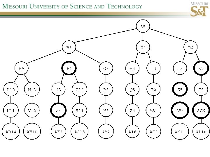
Example state space #2

Graph Search • • • Breadth First Graph Search (BFGS) Uniform Cost Graph Search (UCGS) Depth-First Graph Search (DFGS) Depth-Limited Graph Search (DLGS) Iterative-Deepening Depth-First Graph Search (ID-DFGS)

Best First Search (Be. FS) • Select node to expand based on evaluation function f(n) • Typically node with lowest f(n) selected because f(n) correlated with path-cost • Represent frontier with priority queue sorted in ascending order of f-values

Path-cost functions • g(n) = lowest path-cost from start node to node n • h(n) = estimated path-cost of cheapest path from node n to a goal node [with h(goal)=0]

Heuristics • h(n) is a heuristic function • Heuristics incorporate problemspecific knowledge • Heuristics need to be relatively efficient to compute

Important Be. FS algorithms • UCS: f(n) = g(n) • GBe. FS: f(n) = h(n) • A*S: f(n) = g(n)+h(n)

GBe. FTS • Incomplete (so also not optimal) • Worst-case time and space complexity: O(bm) • Actual complexity depends on accuracy of h(n)

A*S • f(n) = g(n) + h(n) • f(n): estimated cost of optimal solution through node n • if h(n) satisfies certain conditions, A*S is complete & optimal

Example state space # 3

Admissible heuristics • h(n) admissible if: Example: straight line distance A*TS optimal if h(n) admissible

Consistent heuristics • h(n) consistent if: Consistency implies admissibility A*GS optimal if h(n) consistent

A* search notes • • • Optimally efficient for consistent heuristics Run time is a function of the heuristic error Suboptimal variants Not strictly admissible heuristics A* Graph Search not scalable due to memory requirements

Memory-bounded heuristic search • • • Iterative Deepening A* (IDA*) Recursive Best-First Search (RBFS) IDA* and RBFS don’t use all avail. memory Memory-bounded A* (MA*) Simplified MA* (SMA*) Meta-level learning aims to minimize total problem solving cost

Heuristic Functions • • Effective branching factor Domination Composite heuristics Generating admissible heuristics from relaxed problems

Sample relaxed problem • n-puzzle legal actions: Move from A to B if horizontally or vertically adjacent and B is blank Relaxed problems: (a)Move from A to B if adjacent (b)Move from A to B if B is blank (c) Move from A to B

Generating admissible heuristics The cost of an optimal solution to a relaxed problem is an admissible heuristic for the original problem.

Adversarial Search Environments characterized by: • Competitive multi-agent • Turn-taking Simplest type: Discrete, deterministic, two-player, zero-sum games of perfect information

Search problem formulation • • • S 0: Initial state (initial board setup) Player(s): Actions(s): Result(s, a): Terminal test: game over! Utility function: associates playerdependent values with terminal states

Minimax

Depth-Limited Minimax • State Evaluation Heuristic estimates Minimax value of a node • Note that the Minimax value of a node is always calculated for the Max player, even when the Min player is at move in that node!

Iterative-Deepening Minimax • IDM(n, d) calls DLM(n, 1), DLM(n, 2), …, DLM(n, d) • Advantages: –Solution availability when time is critical –Guiding information for deeper searches

Redundant info example

Alpha-Beta Pruning • α: worst value that Max will accept at this point of the search tree • β: worst value that Min will accept at this point of the search tree • Fail-low: encountered value <= α • Fail-high: encountered value >= β • Prune if fail-low for Min-player • Prune if fail-high for Max-player

DLM w/ Alpha-Beta Pruning Time Complexity • Worst-case: O(bd) • Best-case: O(bd/2) [Knuth & Moore, 1975] • Average-case: O(b 3 d/4)

Move Ordering Heuristics • Knowledge based • Killer Move: the last move at a given depth that caused AB-pruning or had best minimax value • History Table

Example game tree

Example game tree

Search Depth Heuristics • Time based / State based • Horizon Effect: the phenomenon of deciding on a non-optimal principal variant because an ultimately unavoidable damaging move seems to be avoided by blocking it till passed the search depth • Singular Extensions / Quiescence Search

Time Per Move • • Constant Percentage of remaining time State dependent Hybrid

Quiescence Search • When search depth reached, compute quiescence state evaluation heuristic • If state quiescent, then proceed as usual; otherwise increase search depth if quiescence search depth not yet reached • Call format: QSDLM(root, depth, QSdepth), QSABDLM(root, depth, QSdepth, α, β), etc.

QS game tree Ex. 1

QS game tree Ex. 2

Forward pruning • Beam Search (n best moves) • Prob. Cut (forward pruning version of alpha-beta pruning)

Transposition Tables (1) • Hash table of previously calculated state evaluation heuristic values • Speedup is particularly huge for iterative deepening search algorithms! • Good for chess because often repeated states in same search

Transposition Tables (2) • Datastructure: Hash table indexed by position • Element: – State evaluation heuristic value – Search depth of stored value – Hash key of position (to eliminate collisions) – (optional) Best move from position

Transposition Tables (3) • Zobrist hash key – Generate 3 d-array of random 64 -bit numbers (piece type, location and color) – Start with a 64 -bit hash key initialized to 0 – Loop through current position, XOR’ing hash key with Zobrist value of each piece found (note: once a key has been found, use an incremental apporach that XOR’s the “from” location and the “to” location to move a piece)

MTD(f) MTDf(root, guess, depth) { lower = -∞; upper = ∞; do { beta=guess+(guess==lower); guess = ABMax. V(root, depth, beta-1, beta); if (guess<beta) upper=guess; else lower=guess; } while (lower < upper); return guess; } // also needs to return best move

IDMTD(f) IDMTDf(root, first_guess, depth_limit) { guess = first_guess; for (depth=1; depth ≤ depth_limit; depth++) guess = MTDf(root, guess, depth); return guess; } // actually needs to return best move

Adversarial Search in Stochastic Environments Worst Case Time Complexity: O(bmnm) with b the average branching factor, m the deepest search depth, and n the average chance branching factor

Example “chance” game tree

Expectiminimax & Pruning • Interval arithmetic • Monte Carlo simulations (for dice called a rollout)

Null Move Forward Pruning • Before regular search, perform shallower depth search (typically two ply less) with the opponent at move; if beta exceeded, then prune without performing regular search • Sacrifices optimality for great speed increase

Futility Pruning • If the current side to move is not in check, the current move about to be searched is not a capture and not a checking move, and the current positional score plus a certain margin (generally the score of a minor piece) would not improve alpha, then the current node is poor, and the last ply of searching can be aborted. • Extended Futility Pruning • Razoring

State-Space Search • • Complete-state formulation Objective function Global optima Local optima (don’t use textbook’s definition!) • Ridges, plateaus, and shoulders • Random search and local search

Steepest-Ascent Hill-Climbing • Greedy Algorithm - makes locally optimal choices Example 8 queens problem has 88≈17 M states SAHC finds global optimum for 14% of instances in on average 4 steps (3 steps when stuck) SAHC w/ up to 100 consecutive sideways moves, finds global optimum for 94% of instances in on average 21 steps (64 steps when stuck)

Stochastic Hill-Climbing • Chooses at random from among uphill moves • Probability of selection can vary with the steepness of the uphill move • On average slower convergence, but also less chance of premature convergence

More Local Search Algorithms • First-choice hill-climbing • Random-restart hill-climbing • Simulated Annealing

Population Based Local Search • • • Deterministic local beam search Stochastic local beam search Evolutionary Algorithms Particle Swarm Optimization Ant Colony Optimization

Particle Swarm Optimization • PSO is a stochastic population-based optimization technique which assigns velocities to population members encoding trial solutions • PSO update rules: PSO demo: http: //www. borgelt. net//psopt. html

Ant Colony Optimization • Population based • Pheromone trail and stigmergetic communication • Shortest path searching • Stochastic moves

Online Search • • Offline search vs. online search Interleaving computation & action Exploration problems, safely explorable Agents have access to: – ACTIONS(s) – c(s, a, s’) – GOAL-TEST(s)

Online Search Optimality • CR – Competitive Ratio • TAPC – Total Actual Path Cost • C* - Optimal Path Cost • Best case: CR = 1 • Worst case: CR = ∞

Online Search Algorithms • Online-DFS-Agent • Random Walk • Learning Real-Time A* (LRTA*)

Online Search Example Graph 1

Online Search Example Graph 2

Online Search Example Graph 3

AI courses at S&T • • CS 345 Computational Robotic Manipulation (SP 2012) CS 347 Introduction to Artificial Intelligence (SP 2012) CS 348 Evolutionary Computing (FS 2011) CS 434 Data Mining & Knowledge Discovery (FS 2011) CS 447 Advanced Topics in AI (SP 2013) CS 448 Advanced Evolutionary Computing (SP 2012) Cp. E 358 Computational Intelligence (FS 2011) Sys. Eng 378 Intro to Neural Networks & Applications