Artificial Intelligence Introduction to Artificial Intelligence AI Many

Artificial Intelligence

Introduction to Artificial Intelligence (AI) • Many applications for AI – Computer vision, natural language processing, speech recognition, search … • But games are some of the more interesting • Opponents that are challenging, or allies that are helpful – Unit that is credited with acting on own • Human-level intelligence too hard – But under narrow circumstances can do pretty well (ex: chess and Deep Blue) – For many games, often constrained (by game rules) • Artificial Intelligence (around in CS for some time)

AI for CS different than AI for Games • Must be smart, but purposely flawed – Loose in a fun, challenging way • No unintended weaknesses – No “golden path” to defeat – Must not look dumb • Must perform in real time • Often, configurable by designers – Not hard coded by programmer • “Amount” and type of AI for game can vary – RTS needs global strategy, FPS needs modeling of individual units at “footstep” level – RTS most demanding: 3 full-time AI programmers – Puzzle, street fighting: 1 part-time AI programmer

Where to Learn AI at WPI? • IMGD 3000 – – Introduction to idea Whirlwind view of techniques Finite State Machines Basic Pathfinding (A*) • IMGD 4000 – Details on basic game AI commonly used in almost all games • Decision trees • Hierarchical state machines – Advanced game AI used, but only in more sophisticated games • Advanced pathfinding • Behavior trees • IMGD 4100 in 2014 “AI for Interactive Media and Games” – Fuzzy logic – Goal-driven agent behavior • CS 4341 “Artificial Intelligence” – Machine learning – Planning

Outline • • • Introduction Common AI Techniques Promising AI Techniques Pathfinding (A*) Finite State Machines Summary (done) (next)

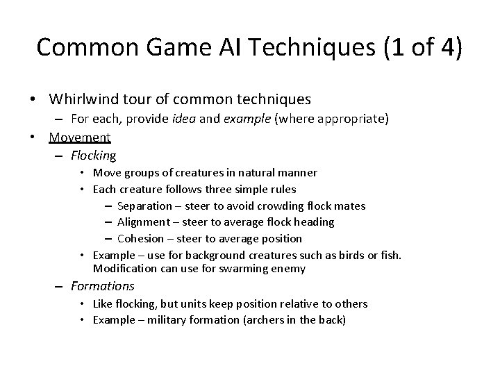
Common Game AI Techniques (1 of 4) • Whirlwind tour of common techniques – For each, provide idea and example (where appropriate) • Movement – Flocking • Move groups of creatures in natural manner • Each creature follows three simple rules – Separation – steer to avoid crowding flock mates – Alignment – steer to average flock heading – Cohesion – steer to average position • Example – use for background creatures such as birds or fish. Modification can use for swarming enemy – Formations • Like flocking, but units keep position relative to others • Example – military formation (archers in the back)

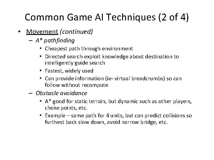
Common Game AI Techniques (2 of 4) • Movement (continued) – A* pathfinding • Cheapest path through environment • Directed search exploit knowledge about destination to intelligently guide search • Fastest, widely used • Can provide information (ie- virtual breadcrumbs) so can follow without recompute – Obstacle avoidance • A* good for static terrain, but dynamic such as other players, choke points, etc. • Example – same path for 4 units, but can predict collisions so furthest back slow down, avoid narrow bridge, etc.

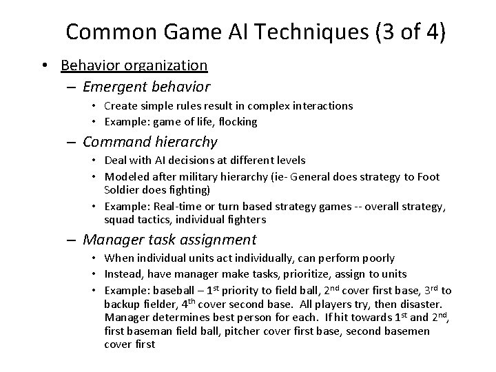
Common Game AI Techniques (3 of 4) • Behavior organization – Emergent behavior • Create simple rules result in complex interactions • Example: game of life, flocking – Command hierarchy • Deal with AI decisions at different levels • Modeled after military hierarchy (ie- General does strategy to Foot Soldier does fighting) • Example: Real-time or turn based strategy games -- overall strategy, squad tactics, individual fighters – Manager task assignment • When individual units act individually, can perform poorly • Instead, have manager make tasks, prioritize, assign to units • Example: baseball – 1 st priority to field ball, 2 nd cover first base, 3 rd to backup fielder, 4 th cover second base. All players try, then disaster. Manager determines best person for each. If hit towards 1 st and 2 nd, first baseman field ball, pitcher cover first base, second basemen cover first

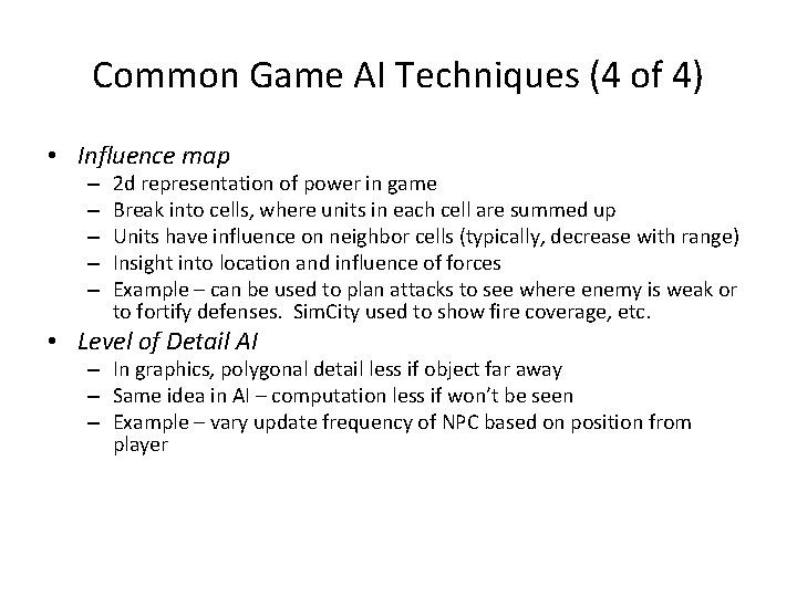
Common Game AI Techniques (4 of 4) • Influence map – – – 2 d representation of power in game Break into cells, where units in each cell are summed up Units have influence on neighbor cells (typically, decrease with range) Insight into location and influence of forces Example – can be used to plan attacks to see where enemy is weak or to fortify defenses. Sim. City used to show fire coverage, etc. • Level of Detail AI – In graphics, polygonal detail less if object far away – Same idea in AI – computation less if won’t be seen – Example – vary update frequency of NPC based on position from player

Outline • • • Introduction Common AI Techniques Promising AI Techniques Pathfinding (A*) Finite State Machines Summary (done) (next)

Promising AI Techniques (1 of 3) • Bayesian network – A probabilistic graphical model with variables and probable influences – Example - calculate probability of patient having a specific disease given symptoms – Example – AI can infer if player has warplanes, etc. based on what it sees in production so far – Can be good to give “human-like” intelligence without cheating or being too dumb • Decision tree learning – Series of inputs (usually game state) mapped to output (usually thing want to predict) – Example – health and ammo predict bot survival – Modify probabilities based on past behavior – Example – Black and White could stroke or slap creature. Creature learned what was good and bad.

Promising AI Techniques (2 of 3) • Filtered randomness – Want randomness to provide unpredictability to AI – But even random can look odd (e. g. - if 4 heads in a row, player think something wrong. And, if flip coin 100 times, will be streak of 8) • E. g. – spawn at same point 5 times in a row, then bad – Compare random result to past history and avoid • Fuzzy logic – Traditional set, object belongs or not. – In fuzzy, can have relative membership (e. g. - hungry, not hungry. Or “in-kitchen” or “in-hall” but what if on edge? ) – Cannot be resolved by coin-flip – Can be used in games – e. g. - assess relative threat

Promising AI Techniques (3 of 3) • Genetic algorithms – Search and optimize based on evolutionary principles – Good when “right” answer not well-understood – E. g. – may not know best combination of AI settings. Use GA to try out – Often expensive, so do offline • N-Gram statistical prediction – Predict next value in sequence (e. g. - 1818180181 … next will probably be 8) – Search backward n values (usually 2 or 3) – Example • Street fighting (punch, kick, low punch…) • Player does low kick and then low punch. What is next? • Uppercut 10 times (50%), low punch (7 times, 35%), sideswipe (3 times, 15%) • Can predict uppercut or, proportionally pick next (e. g. - roll dice)

Outline • • • Introduction Common AI Techniques Promising AI Techniques Pathfinding (A*) Finite State Machines Summary (done) (next)

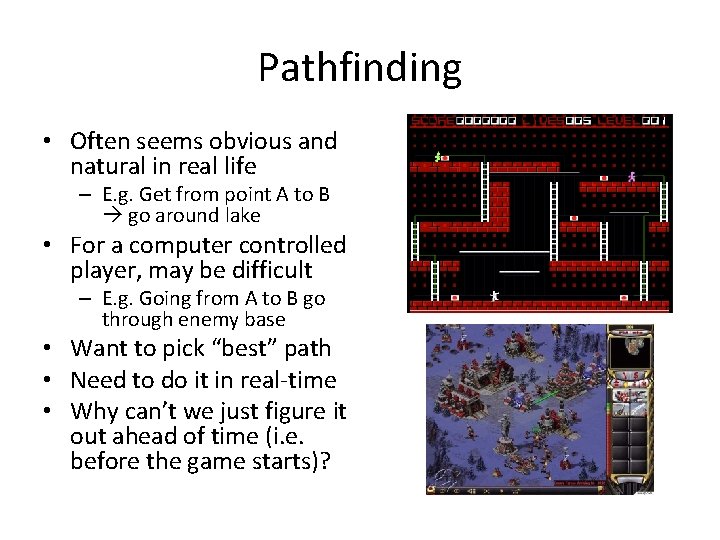
Pathfinding • Often seems obvious and natural in real life – E. g. Get from point A to B go around lake • For a computer controlled player, may be difficult – E. g. Going from A to B go through enemy base • Want to pick “best” path • Need to do it in real-time • Why can’t we just figure it out ahead of time (i. e. before the game starts)?

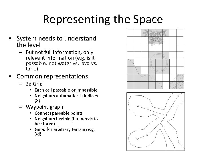
Representing the Space • System needs to understand the level – But not full information, only relevant information (e. g. is it passable, not water vs. lava vs. tar…) • Common representations – 2 d Grid • Each cell passable or impassible • Neighbors automatic via indices (8) – Waypoint graph • Connect passable points • Neighbors flexible (but needs to be stored) • Good for arbitrary terrain (e. g. 3 d)

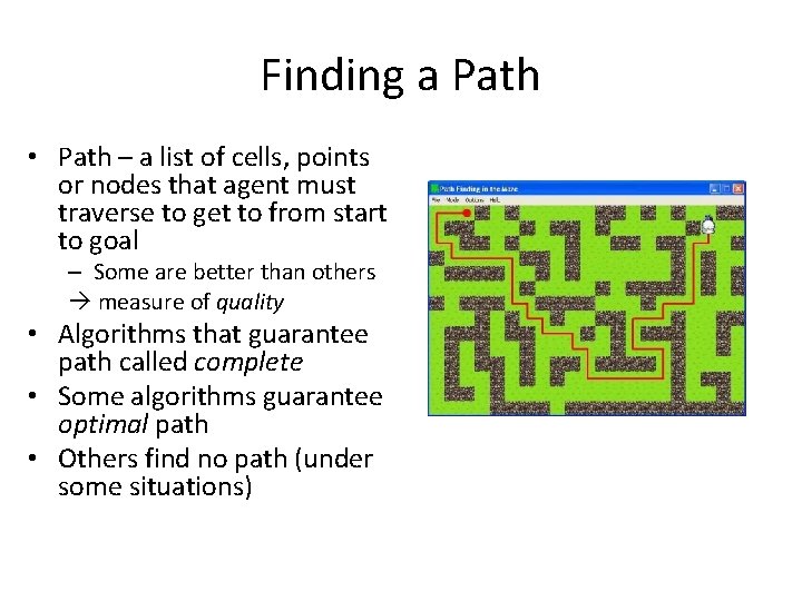
Finding a Path • Path – a list of cells, points or nodes that agent must traverse to get to from start to goal – Some are better than others measure of quality • Algorithms that guarantee path called complete • Some algorithms guarantee optimal path • Others find no path (under some situations)

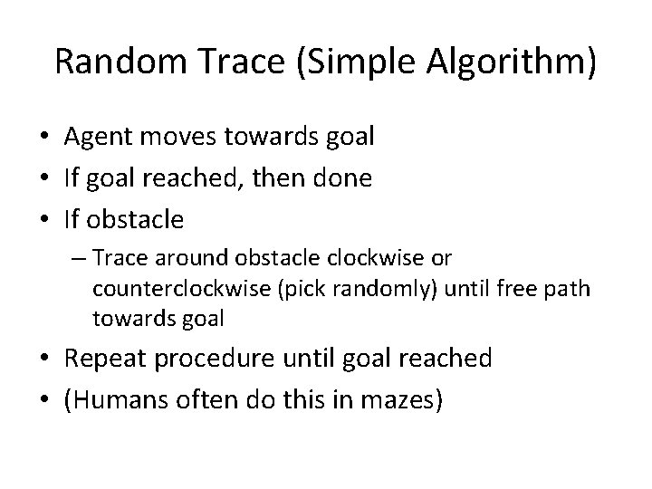
Random Trace (Simple Algorithm) • Agent moves towards goal • If goal reached, then done • If obstacle – Trace around obstacle clockwise or counterclockwise (pick randomly) until free path towards goal • Repeat procedure until goal reached • (Humans often do this in mazes)

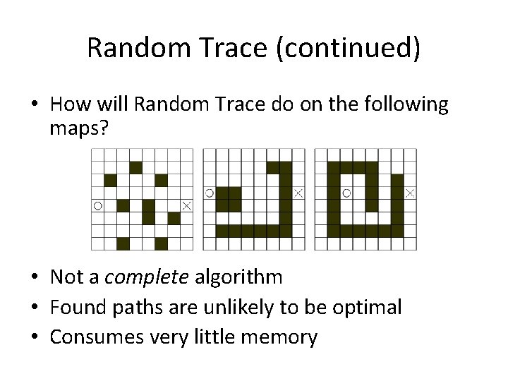
Random Trace (continued) • How will Random Trace do on the following maps? • Not a complete algorithm • Found paths are unlikely to be optimal • Consumes very little memory

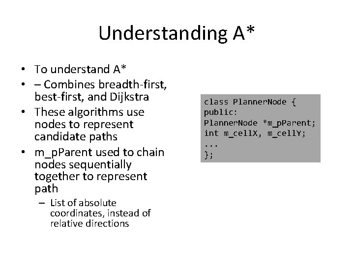
Understanding A* • To understand A* • – Combines breadth-first, best-first, and Dijkstra • These algorithms use nodes to represent candidate paths • m_p. Parent used to chain nodes sequentially together to represent path – List of absolute coordinates, instead of relative directions class Planner. Node { public: Planner. Node *m_p. Parent; int m_cell. X, m_cell. Y; . . . };

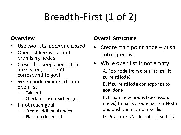
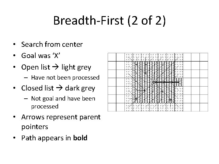
Breadth-First (1 of 2) Overview Overall Structure • Use two lists: open and closed • Open list keeps track of promising nodes • Closed list keeps nodes that are visited, but don’t correspond to goal • When node examined from open list • Create start point node – push onto open list • While open list is not empty – Take off – Check to see if reached goal • If not reach goal – Create additional nodes – Place on closed list A. Pop node from open list (call it current. Node) B. If current. Node corresponds to goal done C. Create new nodes (successors nodes) for cells around current. Node and push them onto open list D. Put current. Node onto closed list

Breadth-First (2 of 2) • Search from center • Goal was ‘X’ • Open list light grey – Have not been processed • Closed list dark grey – Not goal and have been processed • Arrows represent parent pointers • Path appears in bold

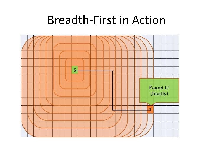
Breadth-First in Action

Breadth-First Characteristics • Exhaustive search • – Systematic, but not clever • Consumes substantial amount of CPU and memory • Guarantees to find paths that have fewest number of nodes in them – Complete algorithm – But not necessarily shortest distance!

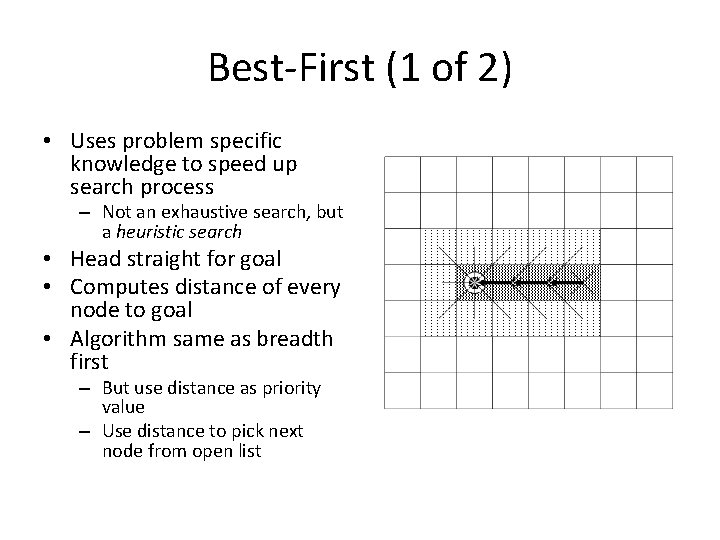
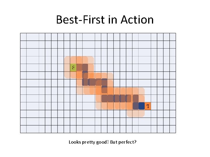
Best-First (1 of 2) • Uses problem specific knowledge to speed up search process – Not an exhaustive search, but a heuristic search • Head straight for goal • Computes distance of every node to goal • Algorithm same as breadth first – But use distance as priority value – Use distance to pick next node from open list

Best-First in Action Looks pretty good! But perfect?

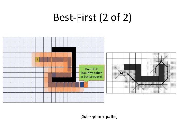
Best-First (2 of 2) (Sub-optimal paths)

Best-First Characteristics • Heuristic search • Uses fewer resources than breadth-first • On average, much faster than breadth-first search • Tends to find good paths – No guarantee to find most optimal path • Complete algorithm

Dijkstra’s Algorithm • Disregards distance to goal – Keeps track of cost of every path – Unlike best-first, no heuristic guessing • Computes accumulated cost paid to reach a node from start – Uses cost (called “given cost”) as priority value to determine next node in open list • Use of cost allows it to handle other terrain – E. g. mud that “slows” or “downhill”

Dijkstra Characteristics • Exhaustive search • At least as resource intensive as Breadth-First • Always finds the optimal path – No algorithm can do better • Complete algorithm

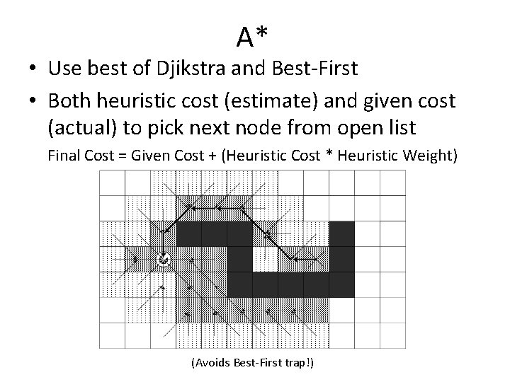
A* • Use best of Djikstra and Best-First • Both heuristic cost (estimate) and given cost (actual) to pick next node from open list Final Cost = Given Cost + (Heuristic Cost * Heuristic Weight) (Avoids Best-First trap!)

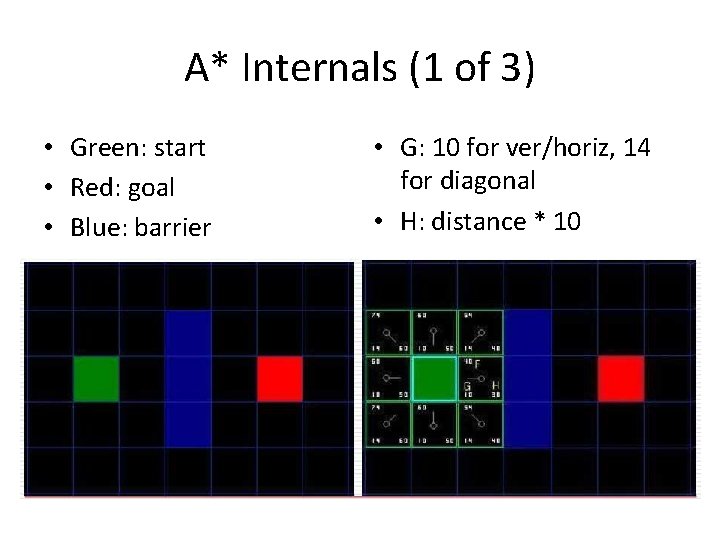
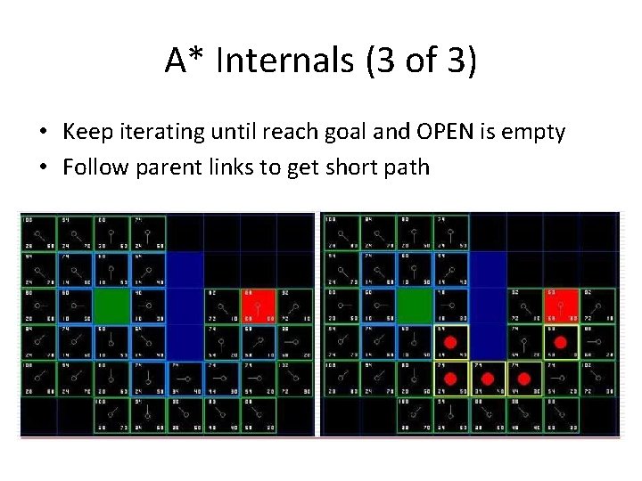
A* Internals (1 of 3) • Green: start • Red: goal • Blue: barrier • G: 10 for ver/horiz, 14 for diagonal • H: distance * 10

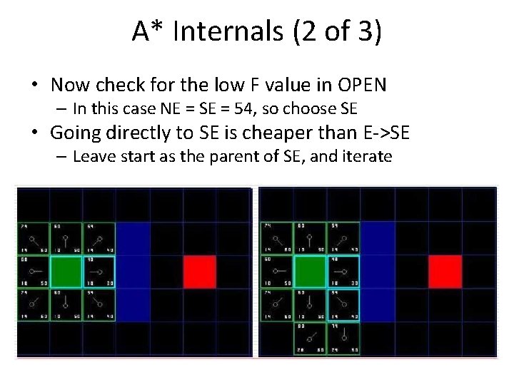
A* Internals (2 of 3) • Now check for the low F value in OPEN – In this case NE = SE = 54, so choose SE • Going directly to SE is cheaper than E->SE – Leave start as the parent of SE, and iterate

A* Internals (3 of 3) • Keep iterating until reach goal and OPEN is empty • Follow parent links to get short path

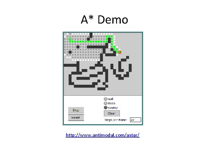
A* Demo http: //www. antimodal. com/astar/

A* Characterisitics • Heuristic search – Weight can control 0 then like Dijkstra, large then like best-first • On average, uses fewer resources than Dijkstra and Breadth-First • “Good” heuristic guarantees it will find the most optimal path – “Good” as long as doesn’t overestimate actual cost – For maps, good is “as a bird flies” distance (best-case) • Complete algorithm

Outline • • • Introduction Common AI Techniques Promising AI Techniques Pathfinding (A*) Finite State Machines Summary (done) (next)

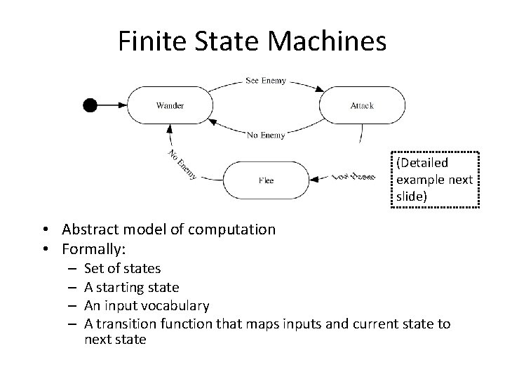
Finite State Machines • Often AI as agents: sense, think, then act • But many different rules for agents – Ex: sensing, thinking and acting when fighting, running, exploring… – Can be difficult to keep rules consistent! • Try Finite State Machine – – – Probably most common game AI software pattern Natural correspondence between states and behaviors Easy: to diagram, program, debug General to any problem See AI Depot - FSM • For each situation, choose appropriate state – Number of rules for each state is small

Finite State Machines (Detailed example next slide) • Abstract model of computation • Formally: – – Set of states A starting state An input vocabulary A transition function that maps inputs and current state to next state

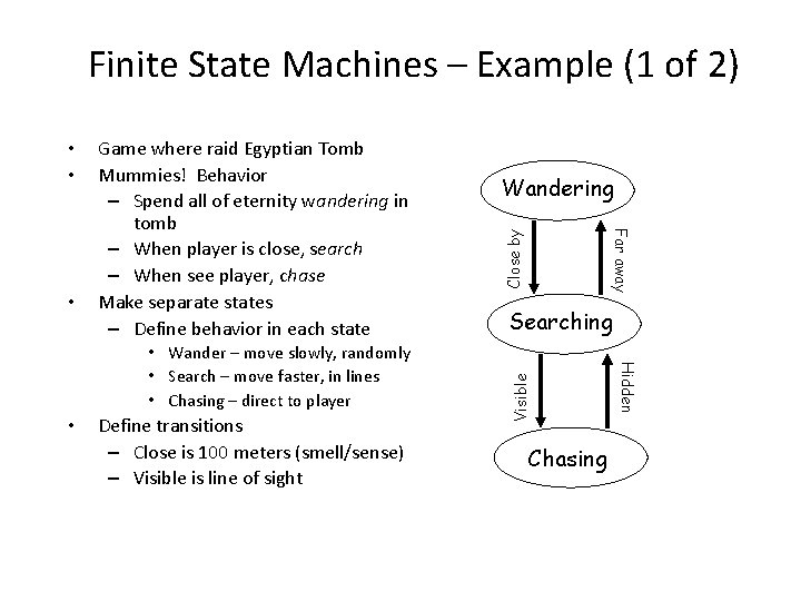
Finite State Machines – Example (1 of 2) • Define transitions – Close is 100 meters (smell/sense) – Visible is line of sight Close by Searching Chasing Hidden • Wander – move slowly, randomly • Search – move faster, in lines • Chasing – direct to player Wandering Far away • Game where raid Egyptian Tomb Mummies! Behavior – Spend all of eternity wandering in tomb – When player is close, search – When see player, chase Make separate states – Define behavior in each state Visible • •

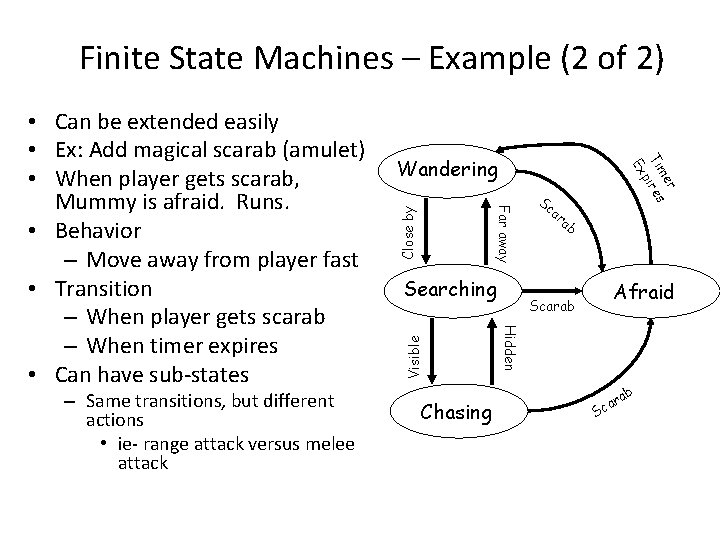
Finite State Machines – Example (2 of 2) Close by Visible Chasing r me Ti ires p Ex Searching Sc ar ab Afraid Scarab Hidden – Same transitions, but different actions • ie- range attack versus melee attack Wandering Far away • Can be extended easily • Ex: Add magical scarab (amulet) • When player gets scarab, Mummy is afraid. Runs. • Behavior – Move away from player fast • Transition – When player gets scarab – When timer expires • Can have sub-states S r ca ab

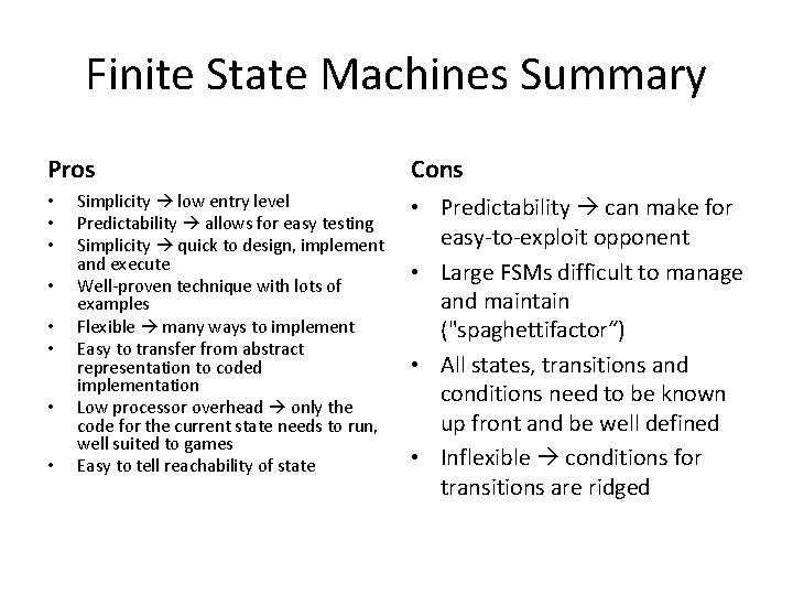
Finite State Machines Summary Pros • • Simplicity low entry level Predictability allows for easy testing Simplicity quick to design, implement and execute Well-proven technique with lots of examples Flexible many ways to implement Easy to transfer from abstract representation to coded implementation Low processor overhead only the code for the current state needs to run, well suited to games Easy to tell reachability of state Cons • Predictability can make for easy-to-exploit opponent • Large FSMs difficult to manage and maintain ("spaghettifactor“) • All states, transitions and conditions need to be known up front and be well defined • Inflexible conditions for transitions are ridged

Summary • AI for games different than other fields – Intelligent opponents, allies and neutral’s but fun (lose in challenging way) – Still, can draw upon broader AI techniques • Finite State Machines flexible, popular – But don’t scale to complicated AI • Dozens of techniques to choose from, with promising techniques on the horizon – AI is the next great “frontier” in games • Two key aspects of pathfinding: – Representing the search space – Searching for a path