Chapter 8 ARTIFICIAL INTELLIGENCE Artificial Intelligence Topics Introduction


 • PSO is a robust stochastic optimization technique")
 • Each particle keeps track of its coordinates in the")
 y x Fig. 1 Concept of modification of a searching")
 • Each particle tries to modify its position using the")
 The following weighting function is usually utilized in (1) w")
 Comments on the Inertial weight factor:")
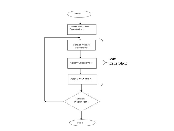
 Flow chart depicting the General PSO Algorithm: Start For each")


 After: (0 1 1 0)")
 (1")


- Slides: 80
Chapter 8 ARTIFICIAL INTELLIGENCE
Artificial Intelligence - Topics • • • • • Introduction to Machine Learning and Artificial Intelligence Expert Systems Biological Neural Networks (BNN) Artificial Neural Networks (ANN) - Fundamentals ANN Characteristics Learning Laws in ANNs Single Layer Perceptrons (SLP) and Multi Layer Perceptrons (MLP) Self Organizing Maps (SOM) Hopfield Associative Memory Adaptive Resonance Theory (ART) Support Vector Machines (SVM) Naïve Bayes Classification- Bayesian Belief Network (BNN) Genetic Algorithm (GA) and Varieties of GA Other Population Based Search Algorithms similar to GA Fuzzy Logic Simulated Annealing
Neural Networks 3
Content • Biological neurons – Axon, dendrites, synaptic • Artificial Neural network • Neuron model • Network topologies – Feed forward – Recurrent – Radial basis function 4
ANN • Ann is an interconnection of simple processing units which communicate by sending signals • Massively parallel • Computational models having the capacity to learn • Learning is achieved by updating the interconnection weights between processing units 5
Neuron model • Receive input from neighbors and/or external sources, use it to compute output • Net input to unit k can be obtained as 6
Neuron model cont… • The output of the neuron is yk • The function Fk is known as activation function • The type of activation function determines the property of the network • Common activation functions 7
Common Activation functions • Smooth and linear functions 8
Network topologies • Neurons can be connected together to form a network • Topology is the way connection is made • In an artificial neural network – Two or more neurons form a layer, neurons with in a layer will have same activation – Layers will be connected to form network – different layers can have different number of neurons and different types of activation 9
Three layer network • The network has input, hidden and output layers • Example : – Hidden layer – tansigmod and output pure linear 10
Network topologies • Feed forward – connection extends from input to output with out any feedback. – Static networks – Used for mapping or function approximation – Example: Perception • Recurrent – contain feedback – Dynamic networks – Example: Hopfield network • Radial basis – feed forward network with bell shaped activation function 11
Training Artificial Neural Network • In a ANN, knowledge is stored in the form connection weights • Hence learning is achieved by adjusting the weights • The process of adjusting the weights is known as training • Paradigms of learning – Supervised learning • Learning by example, input-output pairs or samples will be given to the network and based on the error, weights are adjusted – Unsupervised learning • network finds or searches clusters or patterns in the data without any external agent or teacher 12
Perceptron • Network with threshold activation function • Consider a network with two inputs and one output • If the activation function is hard limiting (threshold) • Then output will be either +1 or -1 13
Example: for the inputs and weights shown determine the outputs x 1 x 2 w 1 w 2 y 0 0 0. 5 -1. 5 1 1 0. 5 -1. 5 1 -1 14
The inverse problem- how to decide the weights values • We want to have the following mapping w 1 w 2 x 1 x 2 y 0 0 -1 0 1 -1 1 0 -1 1 • How to determine the weights? • Learning rules- weights are updated as 15
Hebbian learning rule • Start with random weights • Select an input X from samples • If y d(x), where y is the actual output of the network for input x and d(x) is the desired value, modify the connection as • Go to step 2 16
Example • A perceptron has two inputs and one output. The connection weights are -0. 1 and 0. 5 respectively for the two inputs. The bias is 1. Determine the weights using Hebbian learning rule so that the network implement an OR logic 17
W-H learning rule • Adjust the weights proportional to the error value • Takes less number of iteration and has better convergence 18
Multi-layer feed forward • Two layer feed forward network • Theory of universal approximation – Hidden layer sigmoid – Output layer linear – Can approximate any nonlinear mapping 19
Example • Consider the following input sequence and the networks shown • For a simple feed forward network, with one neuron, linear network with delay and a recurrent network 20
• Simple feed forward network Linear activation p 1 y 0 • Output will be y = [0 0 1 1 1 0 0] 21
• Linear filter, network with input delay Linear activation p 1 y TD 1 0 • Output will be y=[0 0 1 2 2 1 0 0] 22
• Simple recurrent network Linear activation p 1 y 1 0 TD • Output will be y=[0 0 1 2 3 3 3 0] 23
Jordan Network 24
Jordan network It is first proposed in 1986 Its feed back comes from output to input The input from feedback are known as states No. states = No. of output units Connection weight for feedback is constant which is unity • Training is simple • • • – Simple back propagation network is used 25
Elman network 26
Elman network • Introduced in 1990 • Feedback comes from hidden units • In Jordan network, feedback units can have self connection • In Elman network, extra inputs have no self connection • Connection weight for feedback is unity 27
The Hopfield networks • The idea is first proposed by Anderson and Khonon in 1977 • In 1982 Hopfield generalized it • Network contains N interconnected neurons • Connection weight is updated asynchronously and independently • All neurons are both input and output • Activation values are binary (0 and 1 or -1 and 1) 28
Hopfield Network • It is also known as auto associative 29
Hopfield network • If output of a neuron k at time t is Yk, then the net input for neuron k is given by • Where wjk is the connection weight between neuron k and j • The new activation value of the neuron becomes 30
Hopfield network • Stable neuron and stable network – If the output of a neuron remains constant, neuron is said to be stable – The state of the network is the vector Y=(yk) for all k – Stable state – if all neurons are stable at that state – Stable pattern – if network becomes stable for that input 31
Hopfield network • Associative memory – Input pattern and stable state are associated – Hebb learning rule can be used • Hopfield network for optimization – Activation is sigmoid – Neurons are arranged in rows and columns 32
Boltzmann machines • Is extension of Hopfield networks • Works based on principle of annealing • Deterministic output • Stochastic output – probability of becoming active 33
Dynamic networks in MATLAB • Focused time delay networks –newfftd • Distributed time delay networks –newdtdnn • Layered recurrent networks –newlrn 34
Fuzzy logic and its application in Biomedical modeling
Contents • • Fuzzy set theory Fuzzy relations Fuzzy logic control
1 Fuzzy set • Normal set theory allows an element to be a member or not – Universal set U={1 2 3 4 5} – Set A={1 2} – Draw the membership degree as a function of the elements • In fuzzy set an element can be a member to some degree – Fuzzy set • A- the set of all big numbers • B- medium temperature
Degree of membership • In a fuzzy set, the degree of belongingness is expressed in terms of degree of membership • Membership function – A function which maps the Universe of discourse to the numbers in [0 1] – It assigns a number(real) for each element in U • Example – Fuzzy set • A= set of numbers close to 100 1 100
Fuzzy set cont… • For continuous case, possible shapes of mf • For discrete case – Enumeration – Two types of enumeration • Fuzzy set=list in the form of degree of membership/element A=0. 5/1+0. 3/6 • Fuzzy set={(mfv, element 1), (mfv, element 2)…} A={(0. 5, 1), (0. 3, 6)}
2 fuzzy Logic • Some terminologies and symbols – Linguistic variable • Variable expressed in human language • Linguistic description of inputs and outputs • Example: temperature, fault – Linguistic class(values) • Possible divisions of the linguistic variable • Characteristics of the linguistic variable • Hot, cold, medium for temperature – Universe of discourse • The universal set or set containing the complete range of the linguistic variable – Degree of membership – membership value (A)
Fuzzy relations cont… • Union – Union is maximum of membership values For two fuzzy sets A and B, Set(A U B )=max(u(A), u(B)) • Intersection – Is minimum of membership values For two fuzzy sets A and B, Set(A n B )=min(u(A), u(B)) • Complement – 1 -membership value of the given set – Set(A’)=1 -u(A)
Example: Two fuzzy sets A and B are defined as follows • U={ set of positive integers below 10} • A = set of number close to 5 = {0. 1/1+0. 3/2+0. 5/3+0. 8/4+1/5+ 0. 8/6+0. 5/7+0. 3/8+0. 1/9} B=set of small numbers ={1/1+0. 9/2+0. 6/3+0. 4/4+0. 3/5+0. 1/6+0/7+ 0/8+0/9} Find the union, intersection and complement of each set AUB=1/1+0. 9/2+0. 6/3+0. 8/4+1/5+0. 8/6+0. 5/7+ 0. 3/8+0. 1/9 An. B=0. 1/1+0. 3/2+0. 5/3+0. 4/4+0. 3/5+0. 1/6 A’=0. 9/1+0. 7/2+0. 5/3+0. 2/4+0/5+0. 2/6+0. 5/7+…
Fuzzy Rules • Fuzzy rules – Rule base or the linguistic rules define the mapping from input to output – Condition Action – Two types of fuzzy logic systems Type I and Type II Type I: If A is Big then B is small – if part is premise , then part is consequent Type II: If A is Big then B=a. A+b • Max number of rules if there are n inputs, m classes for each input, single outputs, total rules= • Rule derivation – from expert knowledge or characteristic curve
Fuzzy logic control • Parts of a fuzzy logic control
Fuzzification • Is converting crisp inputs to fuzzy set • Usually singleton fuzzification is used • Example: For the following fuzzy set, determine the membership value when input is 0. 5 u(x)=0. 5+2 x/3 -0. 75 x
Inference mechanism • Determines the consequent value based on the given fuzzy rules • Min-max inference mechanism • Two steps – Step 1 - matching – decide which rules are fired – Step 2 - use min-max to decide the consequent fuzzy set
Defuzzification • Determining crisp value from a fuzzy set • Various methods are there • Center of gravity, center of area, centeraverage, height of maxima, height of Area • COG • Center of Area
Applications • Dialysis hypotension control – An automatic system for BP control by fluid removal feedback regulation – Is implemented on dialysis machine – Input is BP – Output- signal that govern ultrafiltration rate(UFR) • Blood glucose regulation
BLOCK DIAGRAM
Evolutionary algorithms and genetic algorithm
Content • • Evolutionary computing and genetic algorithm Evolutionary algorithms Genetic algorithm Application in medical data analysis
Evolutionary computing and genetic algorithm • Is inspired from natural phenomenon • Maps a physical problem into a natural phenomenon • Examples – Particle swarm optimization – Genetic algorithm
Evolutionary algorithms- Particle Swarm Optimization (PSO) • PSO is a robust stochastic optimization technique based on the movement and intelligence of swarms. • PSO applies the concept of social interaction to problem solving. • It was developed in 1995 by James Kennedy (socialpsychologist) and Russell Eberhart (electrical engineer). • It uses a number of agents (particles) that constitute a swarm moving around in the search space looking for the best solution. • Each particle is treated as a point in a N-dimensional space which adjusts its “flying” according to its own flying experience as well as the flying experience of other particles.
Particle Swarm Optimization (PSO) • Each particle keeps track of its coordinates in the solution space which are associated with the best solution (fitness) that has achieved so far by that particle. This value is called personal best , pbest. • Another best value that is tracked by the PSO is the best value obtained so far by any particle in the neighborhood of that particle. This value is called gbest. • The basic concept of PSO lies in accelerating each particle toward its pbest and the gbest locations, with a random weighted accelaration at each time step as shown in Fig. 1
Particle Swarm Optimization (PSO) y x Fig. 1 Concept of modification of a searching point by PSO sk : current searching point. sk+1: modified searching point. vk: current velocity. vk+1: modified velocity. vpbest : velocity based on pbest. vgbest : velocity based on gbest
Particle Swarm Optimization (PSO) • Each particle tries to modify its position using the following information: F the current positions, F the current velocities, F the distance between the current position and pbest, F the distance between the current position and the gbest. • The modification of the particle’s position can be mathematically modeled according the following equation : Vik+1 = w. Vik +c 1 rand 1(…) x (pbesti-sik) + c 2 rand 2(…) x (gbest-sik) …. . (1) where, vik : velocity of agent i at iteration k, w: weighting function, cj : weighting factor, rand : uniformly distributed random number between 0 and 1, sik : current position of agent i at iteration k, pbesti : pbest of agent i, gbest: gbest of the group.
Particle Swarm Optimization (PSO) The following weighting function is usually utilized in (1) w = w. Max-[(w. Max-w. Min) x iter]/max. Iter (2) where w. Max= initial weight, w. Min = final weight, max. Iter = maximum iteration number, iter = current iteration number. sik+1 = sik + Vik+1 (3)
Particle Swarm Optimization (PSO) Comments on the Inertial weight factor:
Particle Swarm Optimization (PSO) Flow chart depicting the General PSO Algorithm: Start For each particle’s position (p) evaluate fitness If fitness(p) better than fitness(pbest) then pbest= p Set best of p. Bests as g. Best Update particles velocity (eq. 1) and position (eq. 3) Stop: giving g. Best, optimal solution. Loop until max iter Loop until all particles exhaust Initialize particles with random position and velocity vectors.
Comparison with other evolutionary computation techniques • Unlike in genetic algorithms, evolutionary programming and evolutionary strategies, in PSO, there is no selection operation. • All particles in PSO are kept as members of the population through the course of the run • PSO is the only algorithm that does not implement the survival of the fittest. • No crossover operation in PSO. • eq 1(b) resembles mutation in EP. • In EP balance between the global and local search can be adjusted through the strategy parameter while in PSO the balance is achieved through the inertial weight factor (w) of eq. 1(a)
Variants of PSO • Discrete PSO ……………… can handle discrete binary variables • MINLP PSO………… can handle both discrete binary and continuous variables. • Hybrid PSO…………. Utilizes basic mechanism of PSO and the natural selection mechanism, which is usually utilized by EC methods such as GAs.
Genetic Algorithm • • • Introduction to Genetic algorithm Basic elements of GA Operators in GA Design of Objective function Multi-objective GA Application in medical data analysis
Introduction to Generic algorithm • Genetic algorithm is an evolutionary algorithm based on Darwin’s theory of selection of the fittest • It is a multidimensional search algorithm which solves the local minima problem of classical algorithms • Basic elements of GA algorithm – Objective function – Gene – Chromosome – Population – Operators
Basic elements of GA • Objective function/ fitness function – The objective to be fulfilled – Constrained or unconstrained objective function – Multiple objective functions can be combined – It may not be differentiable • Gene – in genetics, it is the basic genetic material – In GA based optimization, it is the basic element in a solution of the Objective function – They can be coded as binary or real
Basic elements cont… • Chromosome – is a collection of genes • It represents a candidate solution in the optimization • Example: design the following optimization problem for GA solution Minimize f(x)=x(x-1. 5), we need to find a single variable x Let us assume that we code the genes in binary (1 or 0) and let us assume also that a chromosome will have 4 genes Chromosome 1 = 0010 Chromosome 2 = 0011 Chromosome 3 = 0111
Basic elements cont… • Population – is a collection of chromosomes – Genes- chromosomes- population – Initial population – an initial set of candidate solutions, contains some number of chromosomes • An iteration of GA goes as follows – First a candidate solution or initial population is created – The initial population is tested to see how much the chromosomes in the population fulfill the objective function – Select best chromosomes – Apply operators to create new and better candidates – Repeat the steps
Operators in GA • There are two major operators – Crossover – Mutation • Crossover – Used to mix genetic material of two chromosomes – Pairing is needed – Results in 2 new off springs and 2 parents • Mutation – change in a single chromosome
Mutation: Local Modification Before: (1 0 1 1 0) After: (0 1 1 0) Before: (1. 38 -69. 4 326. 44 0. 1) After: (1. 38 -67. 5 326. 44 0. 1) • Causes movement in the search space (local or global) • Restores lost information to the population
Crossover: Recombination * P 1 P 2 (0 1 1 0 0 0) (1 1 0 1 0) (0 1 0 0 0) (1 1 1 0 1 0) C 1 C 2 Crossover is a critical feature of genetic algorithms: – It greatly accelerates search early in evolution of a population – It leads to effective combination of schemata (subsolutions on different chromosomes)
Cross over for real coding • Discrete – Offspring is selected with equal probability – Example: given parents x and y, off spring z= x or y with equal probability • Intermediate – Single arithmetic – Simple arithmetic – Whole arithmetic
Single arithmetic crossover • • • Parents: x 1, …, xn and y 1, …, yn Pick a single gene (k) at random, child 1 is: • reverse for other child. e. g. with = 0. 5
Simple arithmetic crossover • • • Parents: x 1, …, xn and y 1, …, yn Pick random gene (k) after this point mix values child 1 is: • reverse for other child. e. g. with = 0. 5
Whole arithmetic crossover • • • Most commonly used Parents: x 1, …, xn and y 1, …, yn child 1 is: • reverse for other child. e. g. with = 0. 5
Evaluation evaluated children modified children evaluation • The evaluator decodes a chromosome and assigns it a fitness measure • The evaluator is the only link between a classical GA and the problem it is solving
Deletion population discarded members discard • Generational GA: entire populations replaced with each iteration • Steady-state GA: a few members replaced each generation
Design of objective function • Objective function – GA is designed to maximize a given problem and hence a fitness function has to be designed accordingly – Is the performance index – Determines the effectiveness of the search – Has to be designed carefully – Can be a differentiable or non differentiable function
Simple Genetic Algorithm { initialize population; evaluate population; while Termination. Criteria. Not. Satisfied { select parents for reproduction; perform recombination and mutation; evaluate population; } }
Example: find the solution of the following unconstrained optimization of three variable • Function of two variable • Binary coding - if each gene will be coded with 4 binary digits, for two genes 8 binary digits – Possible chromosome =[01111001] x 1=7 x 2=9 • Real coding – if solution range of x 1 and x 2 is assumed to be [-10 10] – Chromosome =[57] which means x 1=5 and x 2=7
Multi objective GA • Is a GA with multiple objectives – Minimum cost of operation and minimum loss over transmission line • Fitness function has to be designed to represent each objective • Each objective may have its own weight