Connecting Nonlinear Time Series Analysis with Physics Henry

Connecting Nonlinear Time Series Analysis with Physics Henry D. I. Abarbanel Department of Physics and Marine Physical Laboratory (Scripps Institution of Oceanography) University of California, San Diego habarbanel@ucsd. edu

Outline of this talk: I received, via email, a time series of light output from variable stars. This put me into a situation that is a bit awkward for a Physicist who wants to learn about the processes which produced the data and doesn’t know the details about the observations and the instruments used to make them. I do not know the Physics that underlies these data I came here to find out, actually. I do not know the literature on analyzing these time series or anything about the models one uses to describe variable stars.

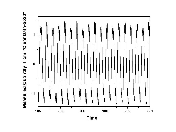
So, violating my moderately strongly held principles about never working with data about which I know nothing, I put on an old, worn engineering hat, and went to work to see if some constraints on any relevant Physics, expressed in a model, could be extracted from the data sent along. ========== Here are some observations about the data I received: The time series has many gaps, and I rejected any tactic to fill in those gaps. I selected one continuous segment of the data from 975 time units to 1000 time units. Δt = 0. 2043 (somethings). The minimum in the data is -1. 34 and the maximum is 1. 57 (not π/2). The mean value is -0. 002, so zero. The data comprises 1211 data points, and it looks like this:

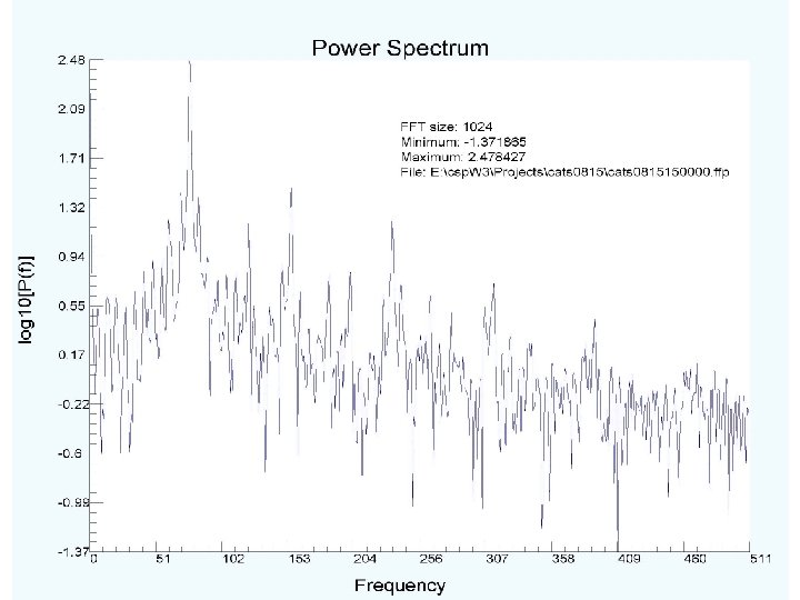
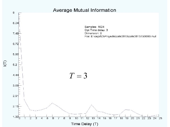
Outline of this talk: It looks close to periodic, but not quite. One would expect there to be a few sharp frequencies in its Fourier spectrum (a linear operation on signals from nonlinear oscillators—but of some use). The “peaks” in the power spectrum should be accompanied by a broadband background. SO: we do the following actions—explanations to accompany the results. Ø examine the Fourier power spectrum; Ø move promptly back to time domain for any further discussion; Ø ask about nonlinear correlations among parts of the data. This is the average mutual information as a function of time lag; Ø select a time lag T where the average mutual information has a first minimum; Ø build from this a “proxy” state space which undoes the projections from the multidimensional phase space where the star’s dynamics happens to the observation axis.

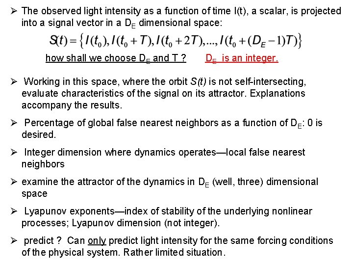
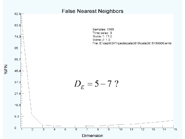
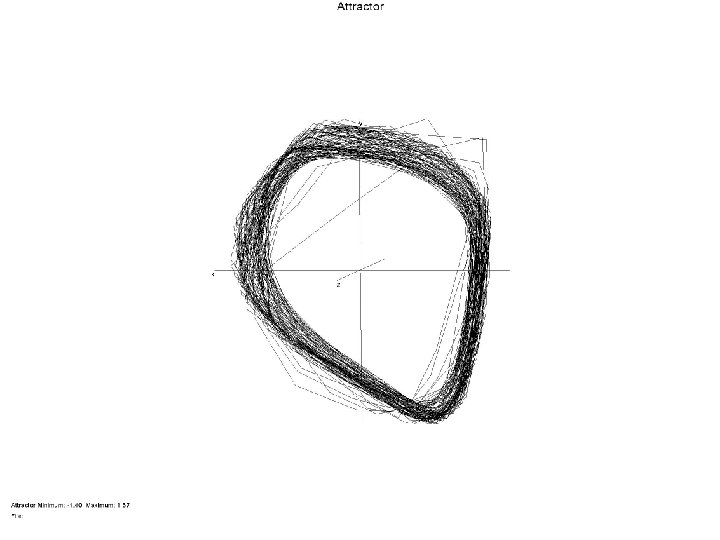
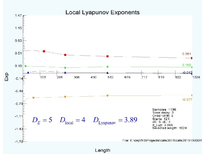
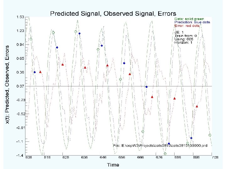
Ø The observed light intensity as a function of time I(t), a scalar, is projected into a signal vector in a DE dimensional space: how shall we choose DE and T ? DE is an integer. Ø Working in this space, where the orbit S(t) is not self-intersecting, evaluate characteristics of the signal on its attractor. Explanations accompany the results. Ø Percentage of global false nearest neighbors as a function of DE: 0 is desired. Ø Integer dimension where dynamics operates—local false nearest neighbors Ø examine the attractor of the dynamics in DE (well, three) dimensional space Ø Lyapunov exponents—index of stability of the underlying nonlinear processes; Lyapunov dimension (not integer). Ø predict ? Can only predict light intensity for the same forcing conditions of the physical system. Rather limited situation.

When we have done all this we will know a small number of characteristics of the processes which produced the signal. These are constraints on the output of any model we make of variable stars. This is not the core Physics. ====== Time to toss the engineering hat and put on the sturdy “get the Physics” hat!

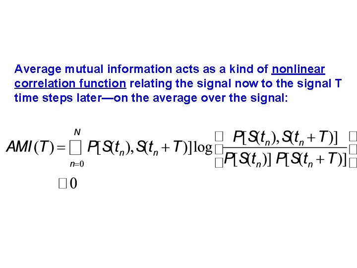
Average mutual information acts as a kind of nonlinear correlation function relating the signal now to the signal T time steps later—on the average over the signal:

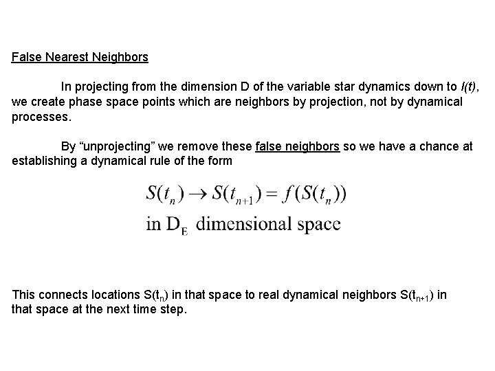
False Nearest Neighbors In projecting from the dimension D of the variable star dynamics down to I(t), we create phase space points which are neighbors by projection, not by dynamical processes. By “unprojecting” we remove these false neighbors so we have a chance at establishing a dynamical rule of the form This connects locations S(tn) in that space to real dynamical neighbors S(tn+1) in that space at the next time step.

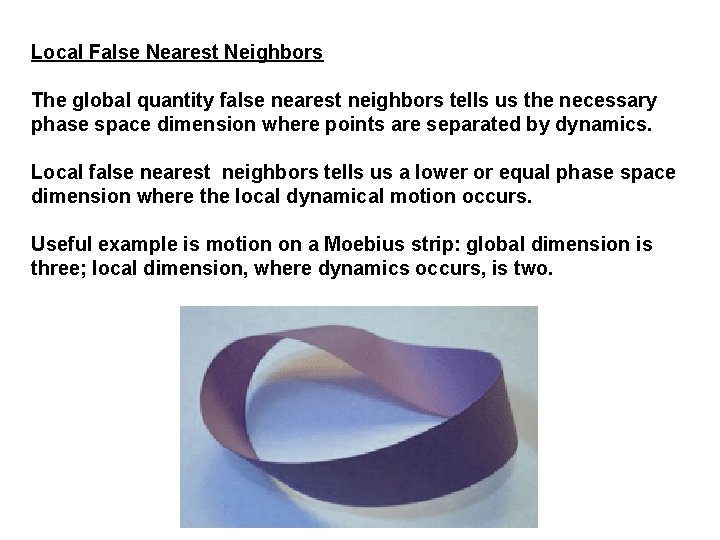
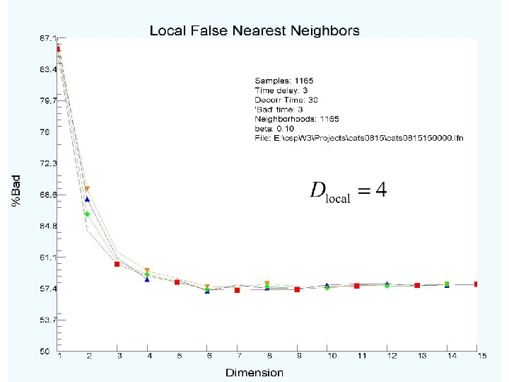
Local False Nearest Neighbors The global quantity false nearest neighbors tells us the necessary phase space dimension where points are separated by dynamics. Local false nearest neighbors tells us a lower or equal phase space dimension where the local dynamical motion occurs. Useful example is motion on a Moebius strip: global dimension is three; local dimension, where dynamics occurs, is two.

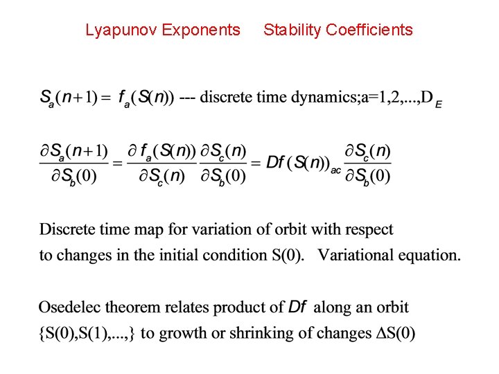
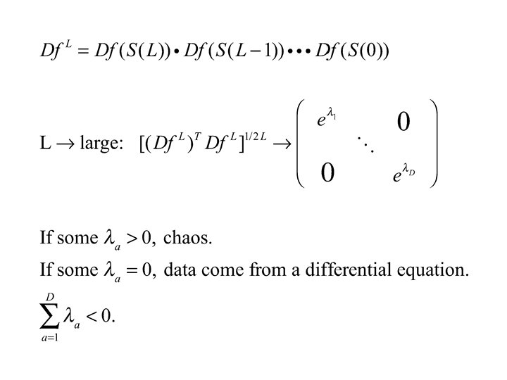
Lyapunov Exponents Stability Coefficients

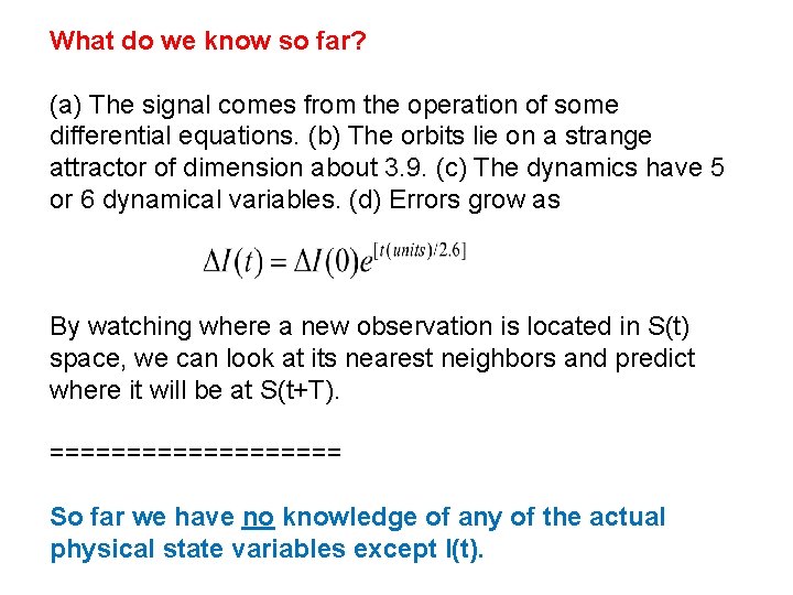
What do we know so far? (a) The signal comes from the operation of some differential equations. (b) The orbits lie on a strange attractor of dimension about 3. 9. (c) The dynamics have 5 or 6 dynamical variables. (d) Errors grow as By watching where a new observation is located in S(t) space, we can look at its nearest neighbors and predict where it will be at S(t+T). ========== So far we have no knowledge of any of the actual physical state variables except I(t).

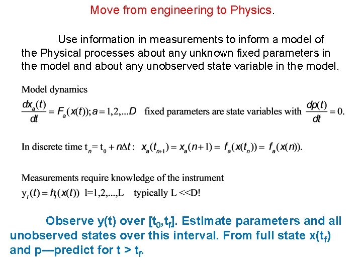
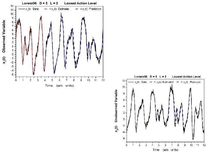
Move from engineering to Physics. Use information in measurements to inform a model of the Physical processes about any unknown fixed parameters in the model and about any unobserved state variable in the model. Observe y(t) over [t 0, tf]. Estimate parameters and all unobserved states over this interval. From full state x(tf) and p---predict for t > tf.

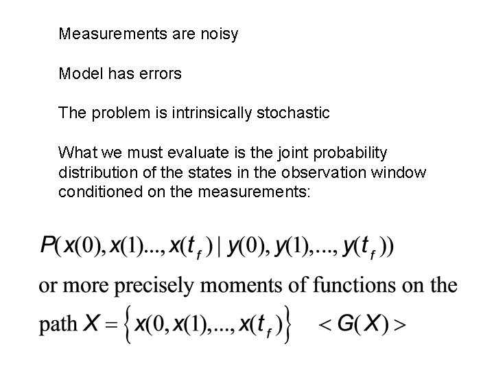
Measurements are noisy Model has errors The problem is intrinsically stochastic What we must evaluate is the joint probability distribution of the states in the observation window conditioned on the measurements:

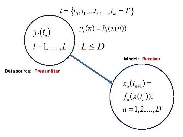
Model: Receiver Data source: Transmitter

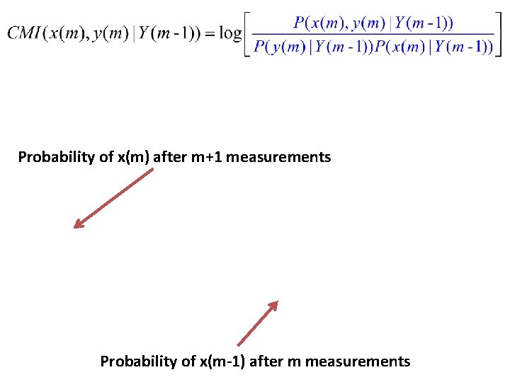
Probability of x(m) after m+1 measurements Probability of x(m-1) after m measurements

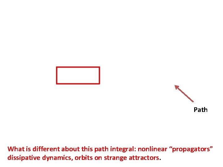
Path What is different about this path integral: nonlinear “propagators” dissipative dynamics, orbits on strange attractors.

Action for State and Parameter Estimation

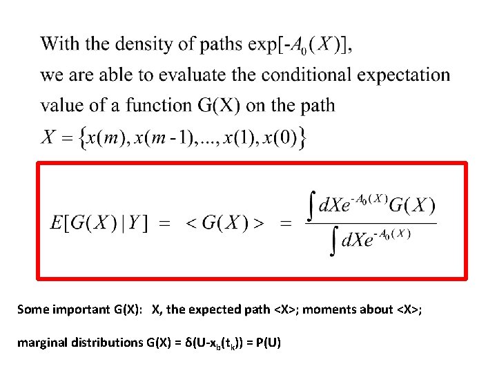
Some important G(X): X, the expected path <X>; moments about <X>; marginal distributions G(X) = δ(U-xb(tk)) = P(U)

Laplace Method for Integrals Variational Methods

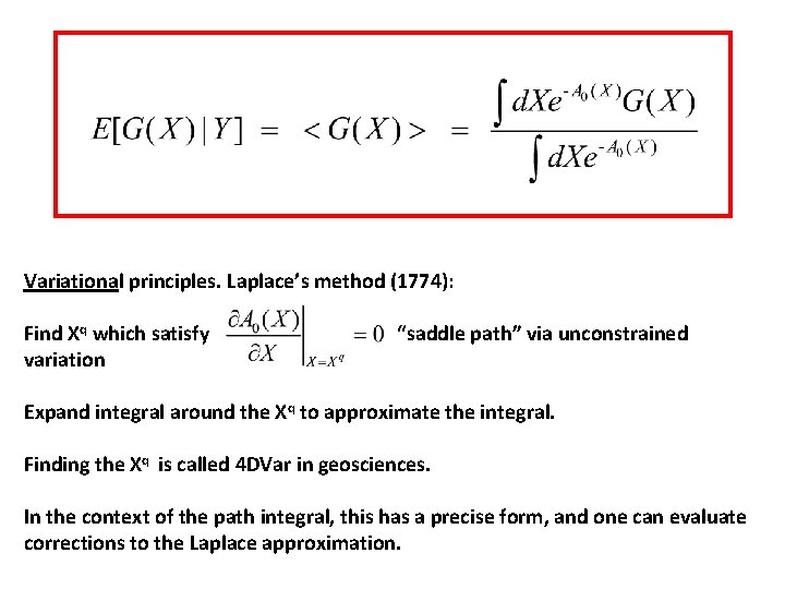
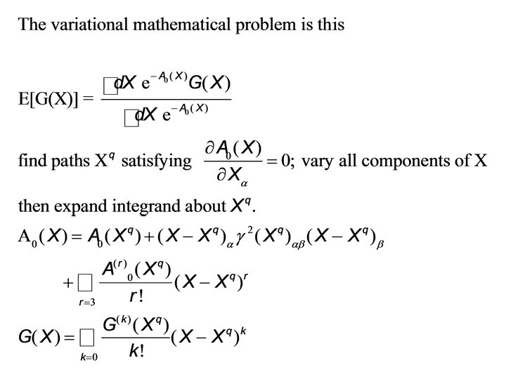
Variational principles. Laplace’s method (1774): Find Xq which satisfy variation “saddle path” via unconstrained Expand integral around the Xq to approximate the integral. Finding the Xq is called 4 DVar in geosciences. In the context of the path integral, this has a precise form, and one can evaluate corrections to the Laplace approximation.

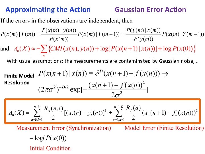
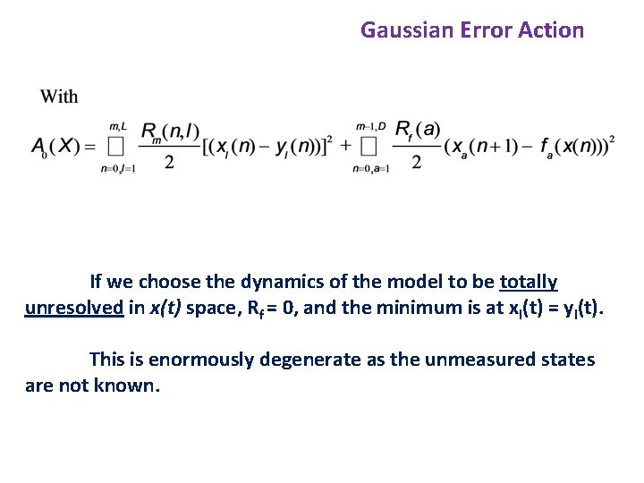
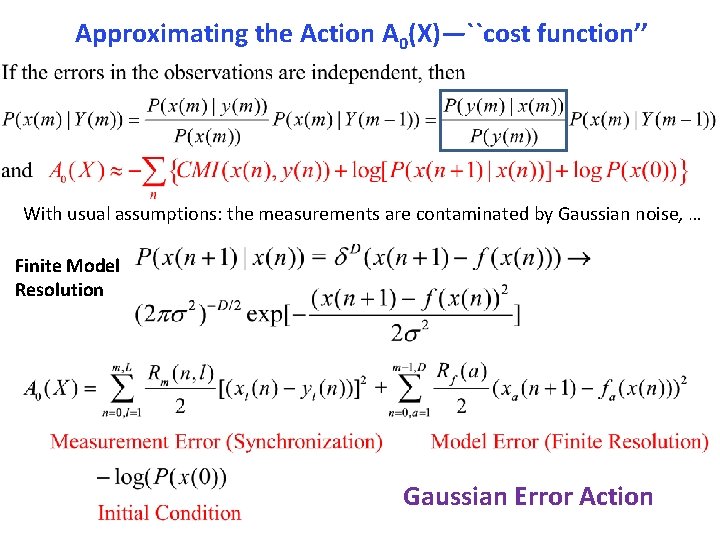
Approximating the Action Gaussian Error Action With usual assumptions: the measurements are contaminated by Gaussian noise, … Finite Model Resolution

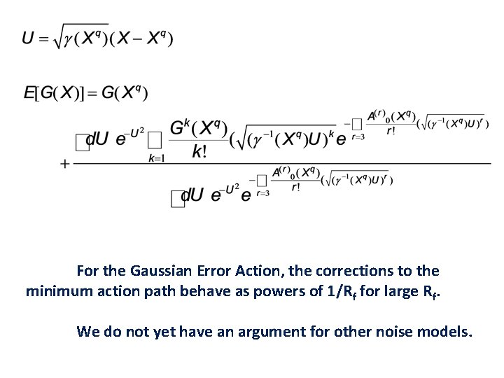
For the Gaussian Error Action, the corrections to the minimum action path behave as powers of 1/Rf for large Rf. We do not yet have an argument for other noise models.

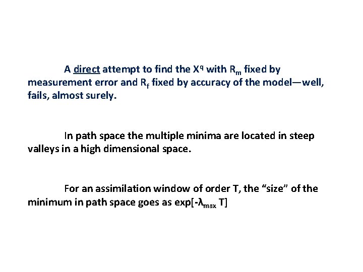
A direct attempt to find the Xq with Rm fixed by measurement error and Rf fixed by accuracy of the model—well, fails, almost surely. In path space the multiple minima are located in steep valleys in a high dimensional space. For an assimilation window of order T, the “size” of the minimum in path space goes as exp[-λmax T]

Gaussian Error Action If we choose the dynamics of the model to be totally unresolved in x(t) space, Rf = 0, and the minimum is at xl(t) = yl(t). This is enormously degenerate as the unmeasured states are not known.

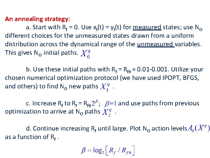
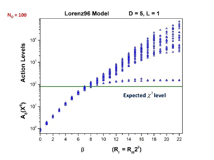
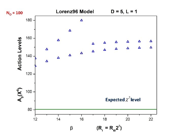
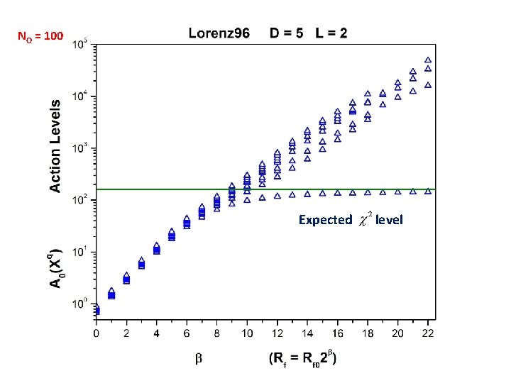
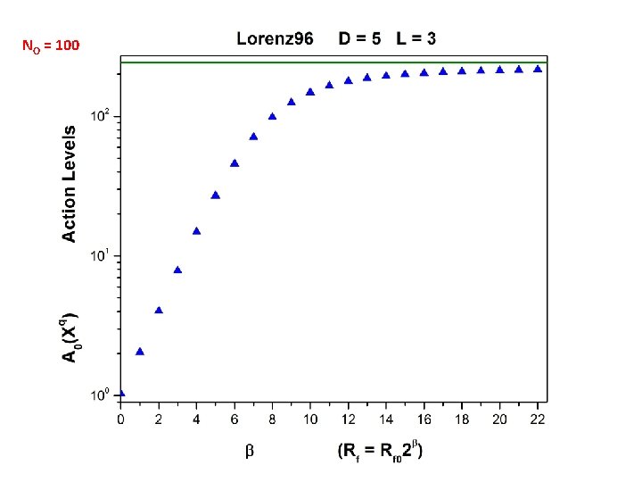
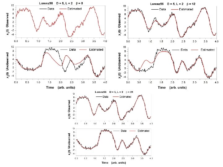
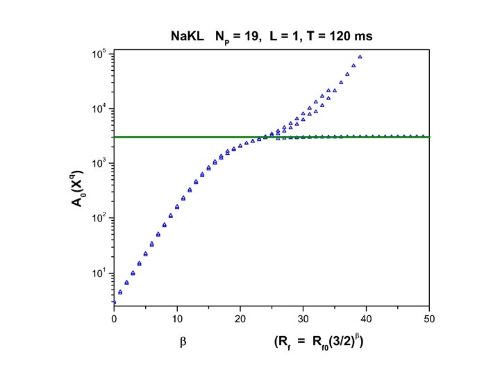
An annealing strategy: a. Start with Rf = 0. Use xl(t) = yl(t) for measured states; use NO different choices for the unmeasured states drawn from a uniform distribution across the dynamical range of the unmeasured variables. This gives NO initial paths. b. Use these initial paths with Rf = Rf 0 ≈ 0. 01 -0. 001. Utilize your chosen numerical optimization protocol (we have used IPOPT, BFGS, and others) to find NO new paths. c. Increase Rf to Rf = Rf 0 optimization to arrive at NO paths . and use paths from previous d. Continue increasing Rf until large. Plot NO action levels as a function of Rf.

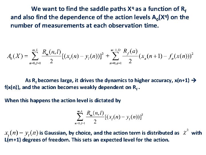
We want to find the saddle paths Xq as a function of Rf and also find the dependence of the action levels A 0(Xq) on the number of measurements at each observation time. As Rf becomes large, it drives the dynamics to higher accuracy, x(n+1) f(x(n)), and the action becomes weakly dependent on Rf. When this happens the action level is dictated by is Gaussian, by choice, and the action term is distributed as L(m+1) degrees of freedom. This sets an expected level for the action. with

We explored D = 5. Chaotic at Forcing = 7. 9; we used Forcing = 8. 17

Model does not synchronize with ‘data’ (x(t)) with only one coupling: two positive Conditional Lyapunov Exponents two different couplings for data are required

NO = 100 Expected level

NO = 100 Expected level

NO = 100 Expected level

NO = 100

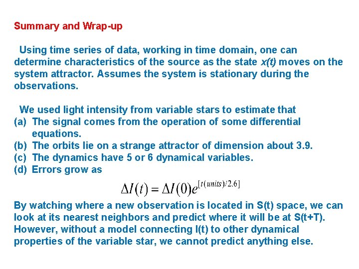
Summary and Wrap-up Using time series of data, working in time domain, one can determine characteristics of the source as the state x(t) moves on the system attractor. Assumes the system is stationary during the observations. We used light intensity from variable stars to estimate that (a) The signal comes from the operation of some differential equations. (b) The orbits lie on a strange attractor of dimension about 3. 9. (c) The dynamics have 5 or 6 dynamical variables. (d) Errors grow as By watching where a new observation is located in S(t) space, we can look at its nearest neighbors and predict where it will be at S(t+T). However, without a model connecting I(t) to other dynamical properties of the variable star, we cannot predict anything else.

Summary and Wrap-up Using the path integral formulation, estimate the conditional expected value of functions along the path. Expectation is conditioned on measurements. Use Laplace approximation or Monte-Carlo approximation of the high dimensional integrals. Require knowledge of the measurements and their relation to the state variables x(t) of the Physics in the model.

Summary and Wrap-up Good “fits” to the observations are unrevealing about the unobserved state variables and the unknown parameters. One critical question is this: how many measurements must be made at each observation time? This is closely related to the positive conditional Lyapunov exponents which control stability. Prediction, deterministic or stochastic, is the key validation of the model. Response to new forcing validates the Physics.

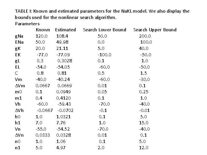
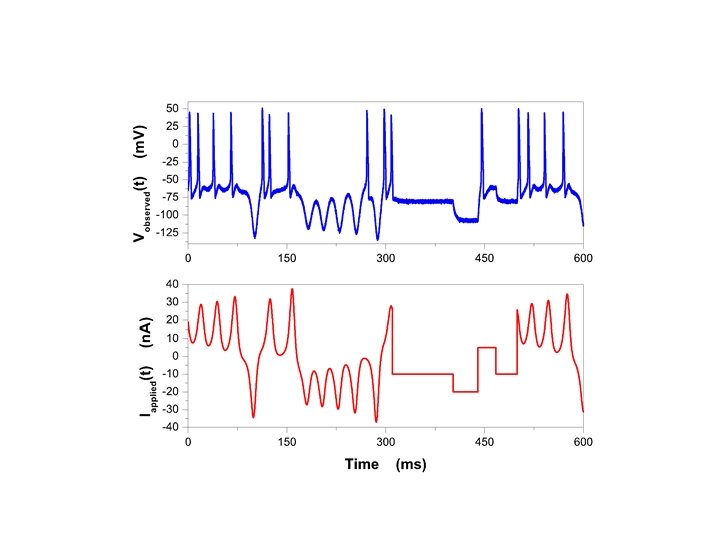
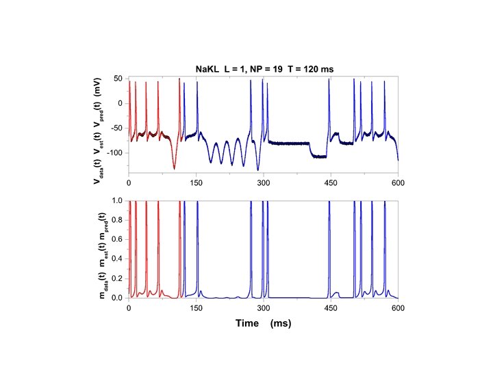
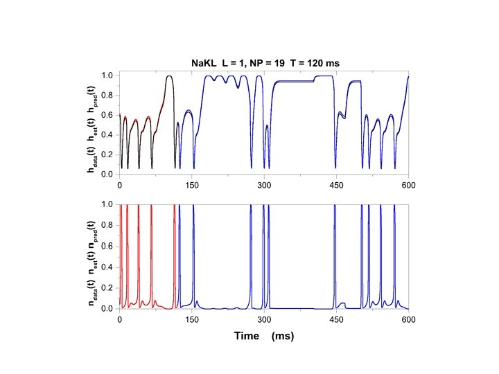
TABLE I: Known and estimated parameters for the Na. KL model. We also display the bounds used for the nonlinear search algorithm. Parameters Known Estimated Search Lower Bound Search Upper Bound g. Na 120. 0 108. 4 50. 0 200. 0 ENa 50. 0 49. 98 0. 0 100. 0 g. K 20. 0 21. 11 5. 0 40. 0 EK -77. 09 -100. 0 -50. 0 g. L 0. 3028 0. 1 1. 0 EL -54. 05 -60. 0 -50. 0 C 0. 81 0. 5 1. 5 Vm -40. 0 -40. 24 -60. 0 -30. 0 ΔVm 0. 0667 0. 0669 0. 01 0. 1 m 0 0. 1 0. 0949 0. 05 0. 25 m 1 0. 4120 0. 1 1. 0 Vh -60. 0 -59. 43 -70. 0 -40. 0 ΔVh -0. 0667 -0. 0702 -0. 1 -0. 01 h 0 1. 0321 0. 1 5. 0 h 1 7. 0 7. 76 1. 0 15. 0 Vn -55. 0 -54. 52 -70. 0 -40. 0 ΔVn 0. 0333 0. 0328 0. 01 0. 1 n 0 1. 06 0. 1 5. 0 n 1 5. 0 4. 97 2. 0 12. 0

Approximating the Action A 0(X)—``cost function’’ With usual assumptions: the measurements are contaminated by Gaussian noise, … Finite Model Resolution Gaussian Error Action

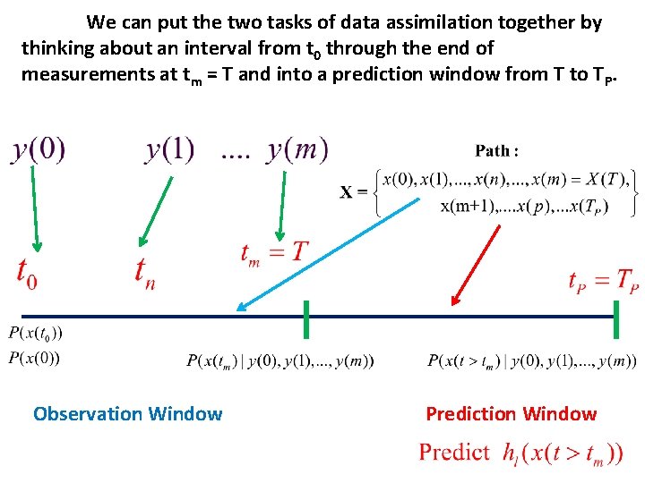
We can put the two tasks of data assimilation together by thinking about an interval from t 0 through the end of measurements at tm = T and into a prediction window from T to TP. Observation Window Prediction Window