Computational Geometry Chapter 14 Line Segments Dealing with

Computational Geometry Chapter 14

Line Segments

Dealing with Degeneracy

Polygons

Convex Polygons

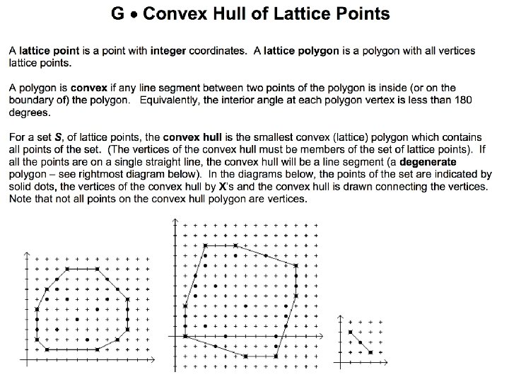
Lattice Points and Pick’s Theorem • Lattice points are unit-spaced grid points. • In general, there will be about one grid point per unit-area in the grid. • The number of grid points within a given figure should give a pretty good approximation to the area of the figure.

Pick’s Theorem • The theorem gives an exact relation between the area of a lattice polygon P (a polygon with the vertices on lattice points) and the number of lattice points on/in the polygon. • Suppose – A(P): area of P – I(P): number of lattice points inside P – B(P): number of lattice points on the boundary of P • The theorem says: A(P) = I(P) + B(P)/2 -1

Pick’s Theorem

Convex Hulls

Convex Hulls • Problems: • Smallest bounding box. • Smallest bounding balls

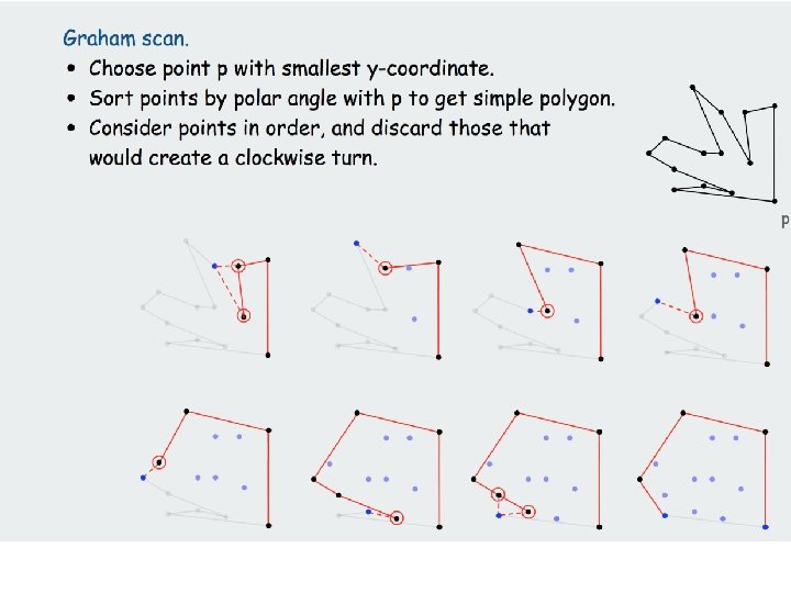
Algorithm to Construct the Convex Hull Given a set S of n points. Construct CH(S), the convex hull of S. The vertices of CH(S) are called extreme points of S. p is an extreme point if an only if it allows a line through p such that all the remaining points strictly lie on one side of the line. • p is an interior point if any line through p splits the point set. The both sides of the line contains points of S. • p is a boundary point if it is not an extreme or an interior point. • •

extreme point interior point boundary point

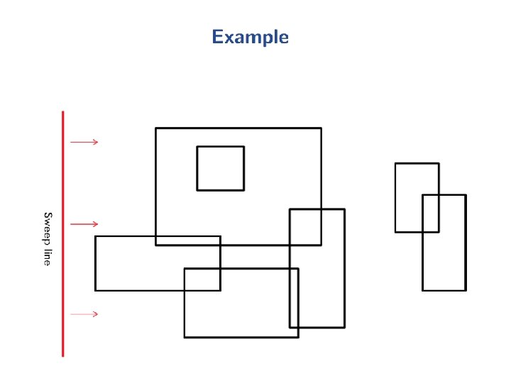
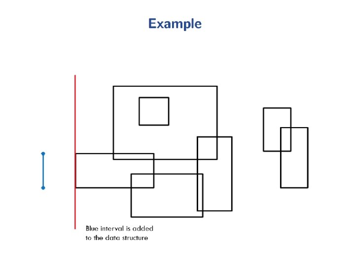
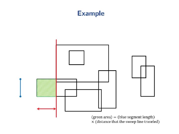
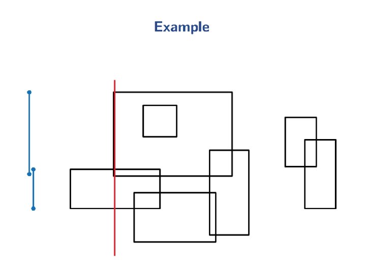
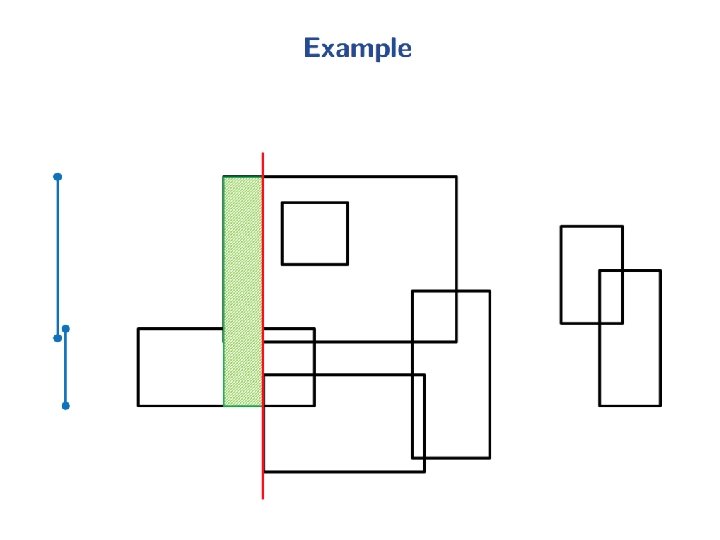
Plane sweep • The idea is to sweep the plane with a line and perform the computations in the sequence the data is encountered. • Can use to construct the convex hull of points

Plane sweep • Can use to construct the convex hull of points • We sweep a vertical line from left to right over the data. • At any moment in time, the points in the front (to the right) are untouched, and the points to the left of the line are already processed.

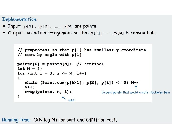
Algorithm to Construct the Convex Hull • Algorithm: – Sort the points by increasing x-order – Let S : <p 1, p 2, …, pn} where pi. x <= pi+1. x for all i. – Let Si = {p 1, p 2, …, pi}, the set of first i points. – Start with the convex hull of the first 3 points p 1, p 2 , p 3. – for i = 4 … n do the following • add the next point pi to te convex hull of the preceding points by finding the two lines that pass through pi and support CH(Si-1).

Illustration: adding p 6

Finding Support Lines • We use a dequeue data structure; a queue-like data structure which allows insertion and deletion of points from both ends. This was discussed in the class. • The dequeue contains the convex hull found so far. The counterclockwise order is obtained by starting from the right end. The clockwise order is obtained by starting from the left end. • For the diagram in the previous slide the content of the dequeue is <…… 5, 4, 3, 2, 5, …>

Finding Support Lines • The effort to insert one point could be large, but it is then we remove many previously added vertices from the list. • We can remove at most n-3 points in total. • Each point gets inserted exactly once. • The total effort to find the supporting linea is therefore O(n).

Algorithm to Construct the Convex Hull • Sorting step costs O(nlogn) • Finding the supporting line step takes linear time. • The convex hull of n points can be computed in O(nlogn) time.

Triangulation • The plane sweep algorithm can be used to decompose the convex hulls into triangles. • Points are never removed. • All we need to change is that instead of deleting the point due to left-right turn of three points, we add the triangle realized by the points of the left-right turn. • The running time is O(n).

Triangulation

Smallest Enclosing Box • Step 1: Compute the convex hull of S. – Let e 1, e 2, …, eh be the edges of the convex hull. • Step 2: For each ei, compute the smallest enclosing box with one side aligned with ei. • Step 3: Report the box with the smallest area. • How quickly can you implement Step 2? – Rotating Caliper Method

Rotating Calipers • A line L is a line of support of a convex polygon P if the interior of P lies completely to one side of L. • A pair of vertices p and q is an antipodal pair if it admits parallel lines of support through p and q.

• pi and pj is an antipodal pair (Fig. 1). To generate the next antipodal pair, we consider the angles that the lines of support at pi and pj with edges pipi+1 and pjpj+1 respectively. • Let θi < θj. • When we rotate clockwise, the lines of support, then the next antipodal pair is either (pi , pj+1 ) or (pj, pi+1).

Smallest Enclosing Box We use two pairs of calipers (Fig. 2). L(pi) denote the directed line of support at pi. L(pj), L(pk) and L(pl) are similarly defined. (pi, pj, pk, pl) form a 4 -tuple forming a rectangle containing P. • We then find the next 4 -tuple by rotating the supporting line by an angle θ = min (θi, θj, θk , θl). • We can find all such 4 -tuples in linear time. • The smallest box can be computed in O(nlogn) time. • •

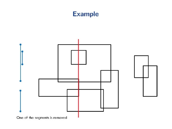
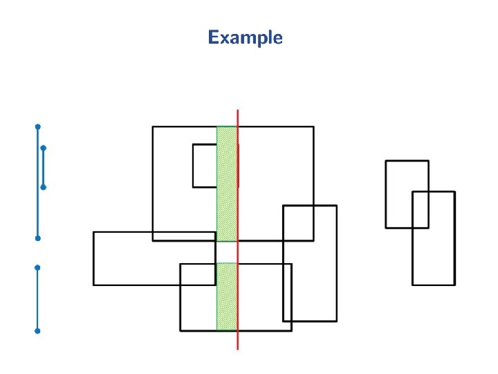
Another sweep line application Slides taken from CS 97 SI --- Stanford U.

Intersection of two Convex Sets Fact 0: Intersection of any two convex sets is convex (possibly empty). Proof: A, B [ (A, B P Q) (A, B P) (A, B Q) (AB P) (AB Q) (AB P Q) ]. P Q B A ax Examples of convex sets: Lines, line segments, convex polygons, half-planes, etc. Line: ax + by = c Half-plane: ax + by c (or ax + by c ) + ax by c ax + by c y= +b c

Intersection of two Convex Polygons Let P and Q be convex polygons with, respectively, n and m vertices. Consider the convex (possibly empty) polygon R = P Q. Fact 1: R has at most n+m vertices. Proof: Let e be any edge of P. e’ = e Q is convex, hence, either empty, a single vertex of Q, or a sub-segment of e. In the latter case e’ is an edge of R. (Similarly, with e an edge of Q and e’ = e P. ) Each edge e of P or Q can contribute at most one such edge e’ to R. P and Q have n and m edges, respectively. Hence, R can have at most n+m edges.

Intersection of two Convex Polygons Fact 2: R = P Q can be computed in O(n+m) time. Proof: Use the plane-sweep method. The upper and lower chains of P and Q are x-monotone (from leftmost to rightmost vertex each). In O(n+m) time, merge these 4 x-sorted vertex-lists to obtain the n+m vertices of P and Q in x-sorted order. This forms the sweep-schedule. These n+m vertical sweep-lines partition the plane into n+m-1 vertical slabs. The intersection of each slab with P or Q is a trapezoid. The two trapezoids within a slab can be intersected in O(1) time. Hence, we can obtain P Q in O(n+m) time. slab

Intersection of n Half-Planes Problem: Given n half-planes H 1, H 2, … , Hn, compute their intersection R = H 1 H 2 … Hn. Input: Hi: ai x + bi y ci , i = 1. . n Output: convex polygon R (empty, bounded or unbounded). R

Intersection of n Half-Planes Problem: Given n half-planes H 1, H 2, … , Hn, compute their intersection R = H 1 H 2 … Hn. Divide-&-Conquer in O(n log n) time: (Use Facts 1 and 2. ) (H 1 … H n/2 ) (H n/2 +1 … Hn Convex P, |P| n/2 T(n/2) time Convex Q, |Q| n/2 T(n/2) time Convex R = P Q, |R| |P|+|Q| n O(n) time T(n) = 2 T(n/2) + O(n) = O(n log n).

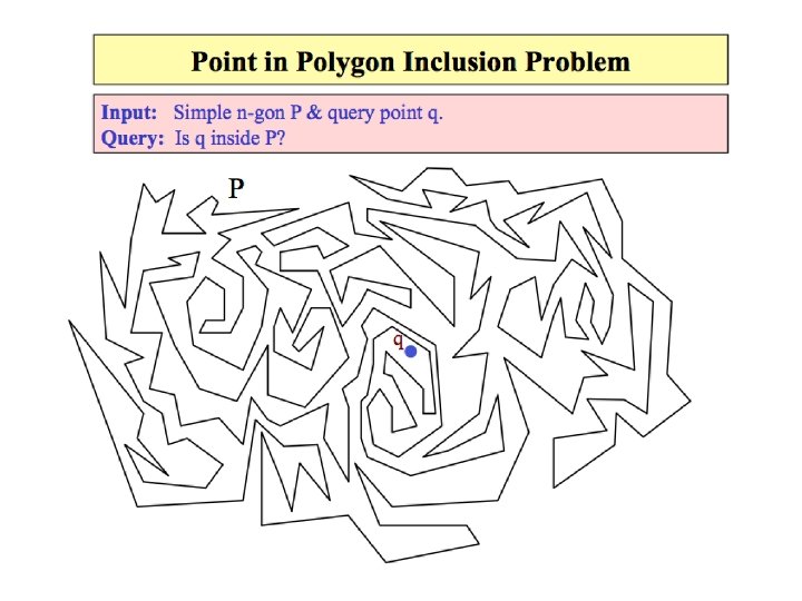
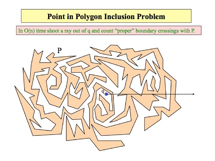
An Art Gallery Problem We are given the floor-plan of an art gallery (with opaque walls) represented by a simple polygon P with n vertices. Is it possible to place a single point camera guard (with 360 vision) in the gallery so that it can “see” every point inside the gallery? q The set of all such points is called the “Kernel” of P. q If Kernel(P) is not empty, then P is called a “star” polygon. P

An Art Gallery Problem We are given the floor-plan of an art gallery (with opaque walls) represented by a simple polygon P with n vertices. Is it possible to place a single point camera guard (with 360 vision) in the gallery so that it can “see” every point inside the gallery? q The set of all such points is called the “Kernel” of P. q If Kernel(P) is not empty, then P is called a “star” polygon. q Kernel(P) is the intersection of n half-planes defined by P’s edges. P

An Art Gallery Problem We are given the floor-plan of an art gallery (with opaque walls) represented by a simple polygon P with n vertices. Is it possible to place a single point camera guard (with 360 vision) in the gallery so that it can “see” every point inside the gallery? q The set of all such points is called the “Kernel” of P. q If Kernel(P) is not empty, then P is called a “star” polygon. q Kernel(P) is the intersection of n half-planes defined by P’s edges. q Kernel(P) can be computed in O(n log n) time by divide-&-conquer. q It can be computed in O(n) time by a careful incremental method that scans the edges of P in order around its boundary. How? P

Range Queries • Orthogonal range queries are a common operation in working with n x m rectilinear grids.

Range Queries • Let pi = (xi, yi), I = 1, 2, 3, 4. • Let m[i][j] = Points (x, y) in the rectangle where x ≥ i and y ≥ j.

Range Queries • Let pi = (xi, yi), I = 1, 2, 3, 4. • Let m[i][j] = Points (x, y) in the rectangle where x ≥ i and y ≥ j. Points inside the rectangle <p 1 p 2 p 3 p 4> = m[x 3][y 3] - m[x 4][y 4] -m[x 2][y 2] +m[x 1][y 1]

Range Queries • Let pi = (xi, yi), I = 1, 2, 3, 4. • Let m[i][j] = Points (x, y) in the rectangle where x ≥ i and y ≥ j. Points inside the rectangle <p 1 p 2 p 3 p 4> = m[x 3][y 3] - m[x 4][y 4] -m[x 2][y 2] +m[x 1][y 1] We can precompute m[i][j] for all values of i and j. --- O(mn) time for an m x n grid.

Data Structure to Store Polygons

Doubly Connected Edge List (DCEL) • DCEL is one of the most commonly used representations for polygons or collection of polygons • It is an edge-based structure which links together the three sets of records: – Vertex – Edge – Face • It facilitates traversing the faces of the collection of polygons visiting all the edges around a given vertex.

Doubly Connected Edge List (DCEL) f 1 f 2 f 4 f 3 edge face f 5 vertex • Record for each face, edge, and vertex – Geometric information – Topological information – Attribute information • Half-edge structure

Doubly Connected Edge List (DCEL) f 1 f 2 f 4 f 3 f 5 • Main ideas: – Edges are oriented counterclockwise inside each face – Since an edge borders two faces, each edge is replaced by two half-edges, one for each face

Doubly Connected Edge List (DCEL) • • • The vertex record of a vertex v stores the coordinates of v. It also stores a pointer Incident. Edge(v) to an arbitrary half-edge that has v as its origin The face record of a face f stores a pointer to some half-edge on its boundary which can be used as a starting point to traverse f in counterclockwise order Incident. Face(e 1) next(e 1) e 2 e 3. twin e 3 e 1 e 4 e 6 e 5 e 4. twin The half-edge record of a half-edge e stores pointer to: • Origin (e) • Twin of e, e. twin or twin(e) • The face to its left ( Incident. Face(e) ) • Next(e) : next half-edge on the boundary of Incident. Face(e) • Previous(e) : previous half-edge origin(e 1) previous(e 1)

Doubly Connected Edge List (DCEL) e 7, 2 v 3 v 6 e 7, 1 e 1, 2 e 5, 1 e 1, 1 f 1 v 1 e 3, 2 e 2, 1 e 5, 2 e 6, 1 f 2 v 4 e 4, 1 e 2, 2 f 3 e 4, 2 v 2 e 6, 2 e 9, 1 e 9, 2 f e 8, 1 4 e 8, 2 v 5 Vertex Coordinates Incident. Edge v 1 (x 1, y 1) e 2, 1 v 2 (x 2, y 2) e 4, 1 v 3 (x 3, y 3) e 3, 2 v 4 (x 4, y 4) e 6, 1 v 5 (x 5, y 5) e 9, 1 v 6 (x 6, y 6) e 7, 1 f 5

Doubly Connected Edge List (DCEL) e 7, 2 v 3 v 6 e 7, 1 e 1, 2 e 5, 1 e 1, 1 v 1 f 1 e 3, 2 e 2, 1 e 5, 2 e 6, 1 f 2 v 4 e 4, 1 e 2, 2 f 3 e 4, 2 e 6, 2 e 9, 1 e 9, 2 f e 8, 1 4 e 8, 2 v 5 v 2 Face Edge f 1 e 1, 1 f 2 e 5, 1 f 3 e 5, 2 f 4 e 8, 1 f 5 e 9, 2 f 5

Doubly Connected Edge List (DCEL) e 7, 2 v 3 v 6 e 7, 1 e 1, 2 e 5, 1 e 1, 1 f 1 v 1 e 3, 2 e 2, 1 e 5, 2 f 3 e 6, 1 f 2 v 4 e 4, 1 e 2, 2 e 4, 2 e 6, 2 e 9, 1 e 9, 2 f 5 f e 8, 1 4 e 8, 2 v 5 v 2 Half-edge Origin Twin Incident. Face Next Previous e 3, 1 v 2 e 3, 2 f 1 e 1, 1 e 2, 1 e 3, 2 v 3 e 3, 1 f 2 e 4, 1 e 5, 1 e 4, 1 v 2 e 4, 2 f 2 e 5, 1 e 3, 2 e 4, 2 v 4 e 4, 1 f 5 e 2, 2 e 8, 2 … … …

Doubly Connected Edge List (DCEL) e 7, 2 v 3 v 6 e 7, 1 e 1, 2 e 5, 1 e 1, 1 v 1 f 1 e 3, 2 e 2, 1 e 5, 2 v 4 e 4, 2 v 2 e 6, 1 f 2 e 4, 1 e 2, 2 f 3 e 6, 2 e 9, 1 e 9, 2 f 5 f e 8, 1 4 e 8, 2 v 5 • Storage space requirement: – Linear in the number of vertices, edges, and faces

Doubly Connected Edge List (DCEL) e 7, 2 v 3 v 6 e 7, 1 e 1, 2 e 5, 1 e 1, 1 f 1 v 1 e 3, 2 e 2, 1 e 5, 2 v 4 e 4, 2 v 2 e 6, 1 f 2 e 4, 1 e 2, 2 f 3 e 6, 2 e 9, 1 e 9, 2 f 5 f e 8, 1 4 e 8, 2 v 5 • Operations: – Walk around the boundary of a given face in CCW order – Access a face from an adjacent one – Visit all the edges around a given vertex

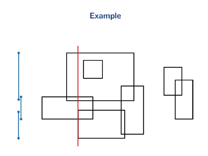
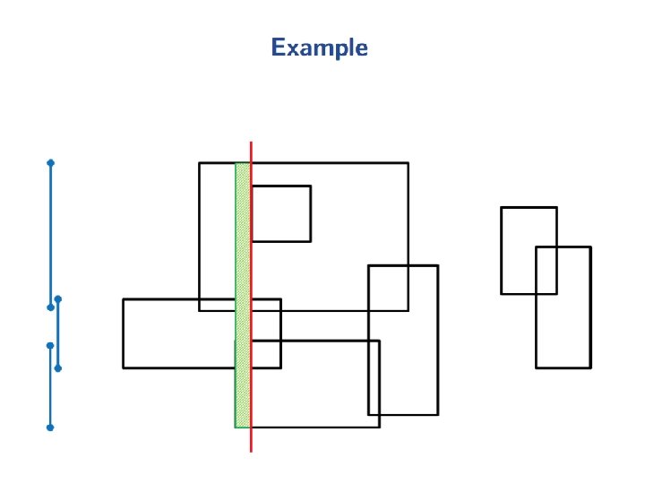
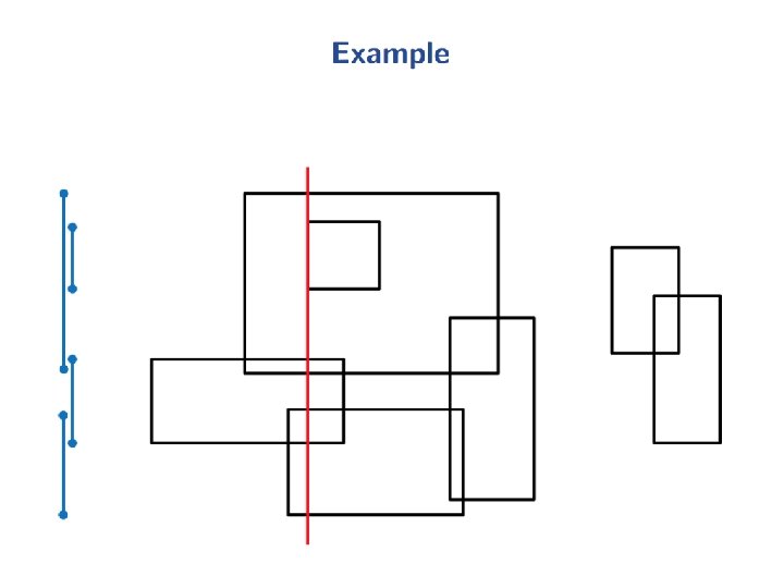
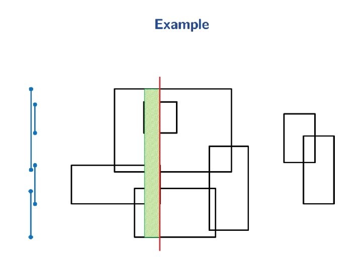
Doubly Connected Edge List (DCEL) e 7, 2 v 3 v 6 e 7, 1 e 1, 2 e 5, 1 e 1, 1 v 1 f 1 e 3, 2 e 2, 1 e 5, 2 e 6, 1 f 2 v 4 e 4, 1 e 2, 2 f 3 e 4, 2 v 2 e 6, 2 e 9, 1 e 9, 2 f 5 f e 8, 1 4 e 8, 2 v 5 • Interesting Queries: – Given a DCEL description, a line L and a half-edge that this line cuts, efficiently find all the faces cut by L.

Doubly Connected Edge List (DCEL) • Traversing face f: – Given: an edge of f 1. Determine the half-edge e incident on f 2. Start_edge e 3. While next(e) start_edge then e next (e)

Doubly Connected Edge List (DCEL) • Traversing all edges incident on a vertex v – Note: we only output the half-edges whose origin is v – Given: a half-edge e with the origin at v 1. Start_edge e 2. While next( twin(e) ) start_edge then e next( twin(e) )

Adding a Vertex (e 1, 2) d = prev ) e 1, 1 a= t( nex e 1, 1 x f 2 e 1, 2 f 1 b = prev(e 1, 1) ) xt(e 1, 2 c = ne

Adding a Vertex • • • New vertex x New edges: e 1, 2’ and e 1, 2’’ Incident. Edge(x) = e 1, 2’ ) e 1, 1 a= • • Origin(e 1, 2’) = x Next(e 1, 2’) = next (e 1, 2) Prev(e 1, 2’) = e 1, 2’’ Incident. Face(e 1, 2’) = f 2 • • Origin(e 1, 2’’) = origin(e 1, 2) Next(e 1, 2’’) = e 1, 2’ Prev(e 1, 2’’) = prev(e 1, 2) Incident. Face(e 1, 2’’) = f 2 • • Next(Prev(e 1, 2)) = e 1, 2’’ Prev(Next(e 1, 2)) = e 1, 2’ • Delete edge e 1, 2 (e 1, 2) d = prev t( nex e 1, 2’’ e 1, 1 f 1 x f 2 e 1, 2’ b = prev(e 1, 1) ) xt(e 1, 2 c = ne

Adding a Vertex • New edges: e 1, 1’ and e 1, 1’’ • • Origin(e 1, 1’) = origin(e 1, 1) Next(e 1, 1’) = e 1, 1’’ Prev(e 1, 1’) = prev(e 1, 1) Incident. Face(e 1, 1’) = f 1 • • Origin(e 1, 1’’) = e 1, 1’ Next(e 1, 1’’) = next(e 1, 1) Prev(e 1, 1’’) = e 1, 1’ Incident. Face(e 1, 1’’) = f 1 • • Next(prev(e 1, 1)) = e 1, 1’ Prev(next(e 1, 1)) = e 1, 1’’ • • • Twin(e 1, 2’) = e 1, 1’ Twin(e 1, 1’) = e 1, 2’ Twin(e 1, 2’’) = e 1, 1’’ Twin(e 1, 1’’) = e 1, 2’’ Delete edge e 1, 1 ) e 1, 1 a= t( nex e 1, 1’’ f 1 (e 1, 2) d = prev e 1, 2’’ x e 1, 1’ f 2 e 1, 2’ b = prev(e 1, 1) ) xt(e 1, 2 c = ne

Adding a Vertex • • If e 1, 1 was starting edge of f 1, need to change it to either one of the new edges If e 1, 2 was starting edge of f 2, need to change it to either one of the new edges ) e 1, 1 a= t( nex e 1, 1’’ f 1 (e 1, 2) d = prev e 1, 2’’ x e 1, 1’ f 2 e 1, 2’ b = prev(e 1, 1) ) xt(e 1, 2 c = ne

Other Operations on DCEL e b a • Add an Edge – Planar subdivision – e is added – DCEL can be updated in constant time once the edges a and b are known