COMP 206 Computer Architecture and Implementation Montek Singh

COMP 206: Computer Architecture and Implementation Montek Singh Wed. , Aug 26, 2002 1

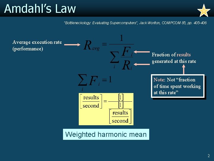
Amdahl’s Law “Bottleneckology: Evaluating Supercomputers”, Jack Worlton, COMPCOM 85, pp. 405 -406 Average execution rate (performance) Fraction of results generated at this rate Note: Not “fraction of time spent working at this rate” Weighted harmonic mean 2

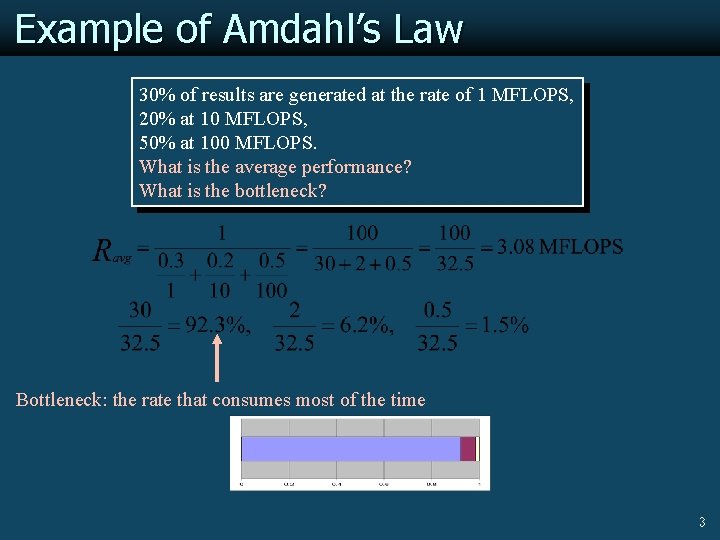
Example of Amdahl’s Law 30% of results are generated at the rate of 1 MFLOPS, 20% at 10 MFLOPS, 50% at 100 MFLOPS. What is the average performance? What is the bottleneck? Bottleneck: the rate that consumes most of the time 3

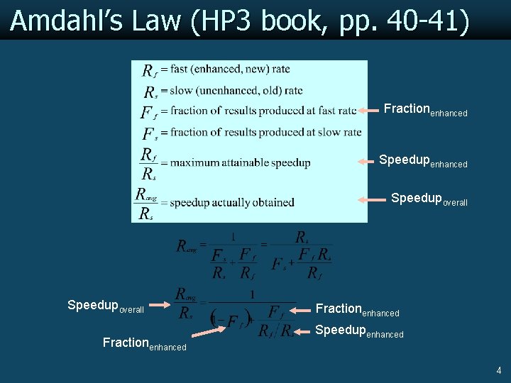
Amdahl’s Law (HP 3 book, pp. 40 -41) Fractionenhanced Speedupoverall Fractionenhanced Speedupenhanced 4

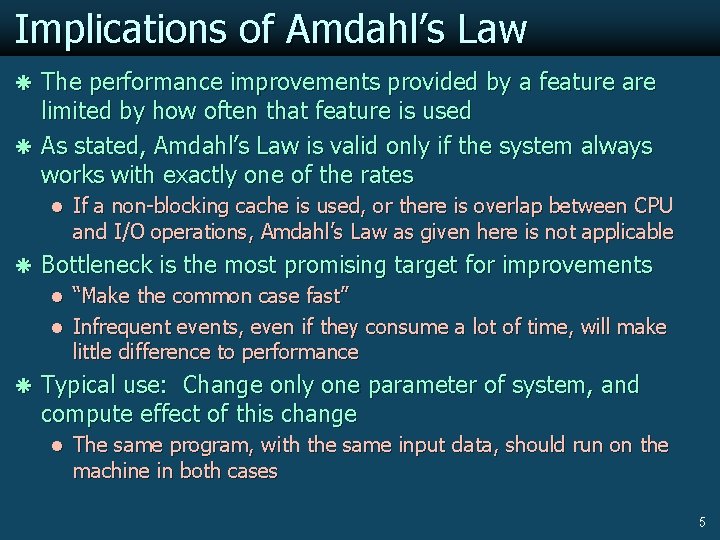
Implications of Amdahl’s Law ã The performance improvements provided by a feature are limited by how often that feature is used ã As stated, Amdahl’s Law is valid only if the system always works with exactly one of the rates l If a non-blocking cache is used, or there is overlap between CPU and I/O operations, Amdahl’s Law as given here is not applicable ã Bottleneck is the most promising target for improvements l “Make the common case fast” l Infrequent events, even if they consume a lot of time, will make little difference to performance ã Typical use: Change only one parameter of system, and compute effect of this change l The same program, with the same input data, should run on the machine in both cases 5

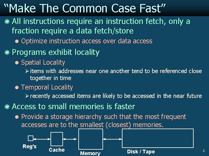
“Make The Common Case Fast” ã All instructions require an instruction fetch, only a fraction require a data fetch/store l Optimize instruction access over data access ã Programs exhibit locality l Spatial Locality Ø items with addresses near one another tend to be referenced close together in time l Temporal Locality Ø recently accessed items are likely to be accessed in the near future ã Access to small memories is faster l Provide a storage hierarchy such that the most frequent accesses are to the smallest (closest) memories. Reg's Cache Memory Disk / Tape 6

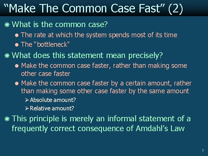
“Make The Common Case Fast” (2) ã What is the common case? l The rate at which the system spends most of its time l The “bottleneck” ã What does this statement mean precisely? l Make the common case faster, rather than making some other case faster l Make the common case faster by a certain amount, rather than making some other case faster by the same amount Ø Absolute amount? Ø Relative amount? ã This principle is merely an informal statement of a frequently correct consequence of Amdahl’s Law 7

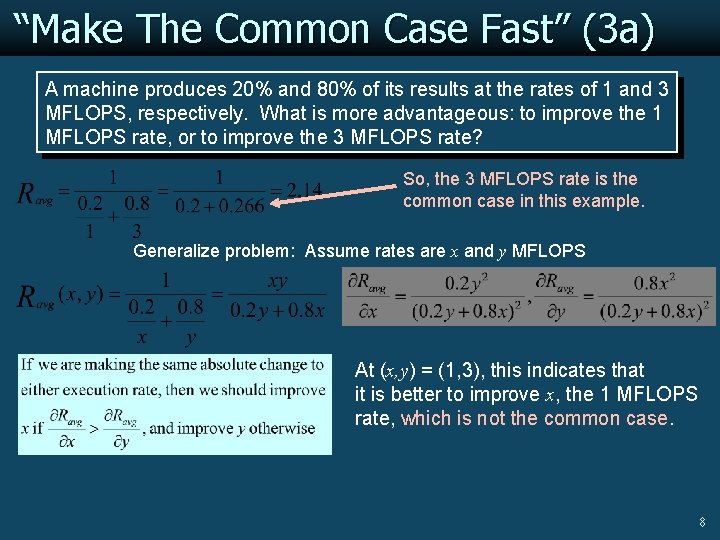
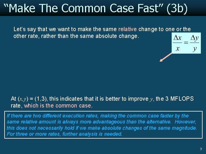
“Make The Common Case Fast” (3 a) A machine produces 20% and 80% of its results at the rates of 1 and 3 MFLOPS, respectively. What is more advantageous: to improve the 1 MFLOPS rate, or to improve the 3 MFLOPS rate? So, the 3 MFLOPS rate is the common case in this example. Generalize problem: Assume rates are x and y MFLOPS At (x, y) = (1, 3), this indicates that it is better to improve x, the 1 MFLOPS rate, which is not the common case. 8

“Make The Common Case Fast” (3 b) Let’s say that we want to make the same relative change to one or the other rate, rather than the same absolute change. At (x, y) = (1, 3), this indicates that it is better to improve y, the 3 MFLOPS rate, which is the common case. If there are two different execution rates, making the common case faster by the same relative amount is always more advantageous than the alternative. However, this does not necessarily hold if we make absolute changes of the same magnitude. For three or more rates, further analysis is needed. 9

Basics of Performance 10

Details of CPI 11

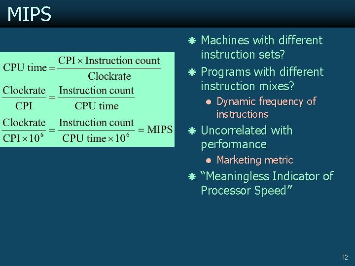
MIPS ã Machines with different instruction sets? ã Programs with different instruction mixes? l Dynamic frequency of instructions ã Uncorrelated with performance l Marketing metric ã “Meaningless Indicator of Processor Speed” 12

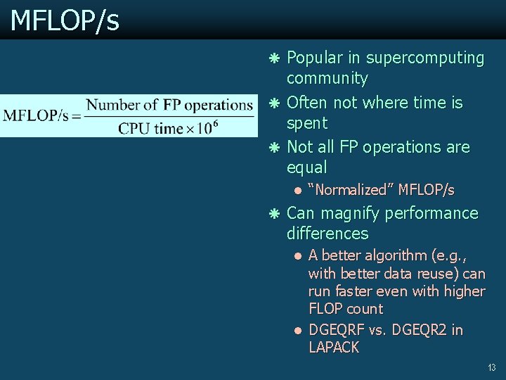
MFLOP/s ã Popular in supercomputing community ã Often not where time is spent ã Not all FP operations are equal l “Normalized” MFLOP/s ã Can magnify performance differences l A better algorithm (e. g. , with better data reuse) can run faster even with higher FLOP count l DGEQRF vs. DGEQR 2 in LAPACK 13

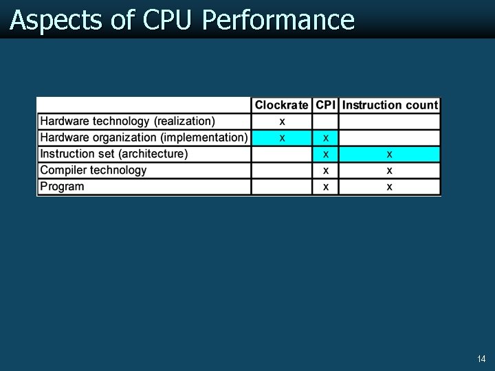
Aspects of CPU Performance 14

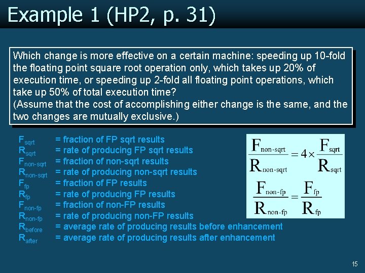
Example 1 (HP 2, p. 31) Which change is more effective on a certain machine: speeding up 10 -fold the floating point square root operation only, which takes up 20% of execution time, or speeding up 2 -fold all floating point operations, which take up 50% of total execution time? (Assume that the cost of accomplishing either change is the same, and the two changes are mutually exclusive. ) Fsqrt Rsqrt Fnon-sqrt Rnon-sqrt Ffp Rfp Fnon-fp Rbefore Rafter = fraction of FP sqrt results = rate of producing FP sqrt results = fraction of non-sqrt results = rate of producing non-sqrt results = fraction of FP results = rate of producing FP results = fraction of non-FP results = rate of producing non-FP results = average rate of producing results before enhancement = average rate of producing results after enhancement 15

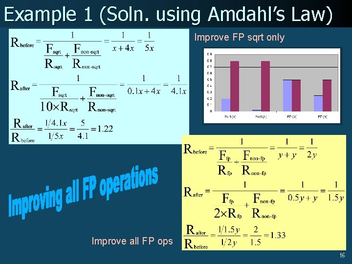
Example 1 (Soln. using Amdahl’s Law) Improve FP sqrt only Improve all FP ops 16

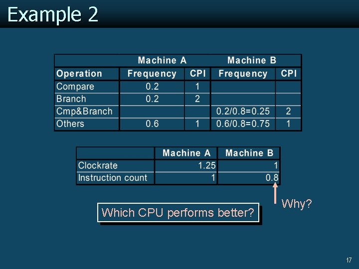
Example 2 Which CPU performs better? Why? 17

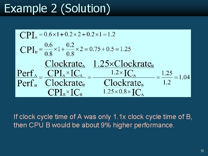
Example 2 (Solution) If clock cycle time of A was only 1. 1 x clock cycle time of B, then CPU B would be about 9% higher performance. 18

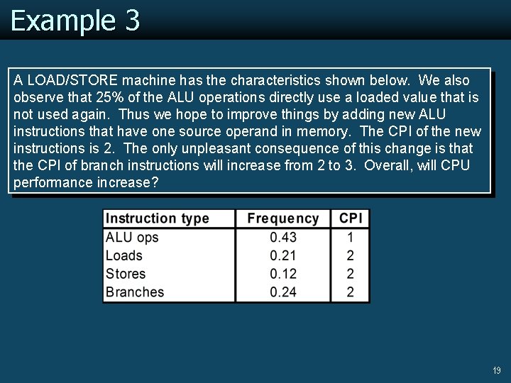
Example 3 A LOAD/STORE machine has the characteristics shown below. We also observe that 25% of the ALU operations directly use a loaded value that is not used again. Thus we hope to improve things by adding new ALU instructions that have one source operand in memory. The CPI of the new instructions is 2. The only unpleasant consequence of this change is that the CPI of branch instructions will increase from 2 to 3. Overall, will CPU performance increase? 19

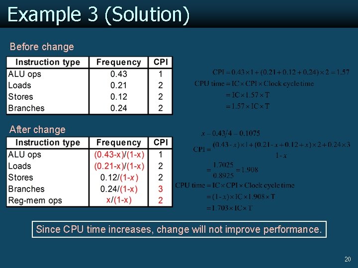
Example 3 (Solution) Before change After change Since CPU time increases, change will not improve performance. 20

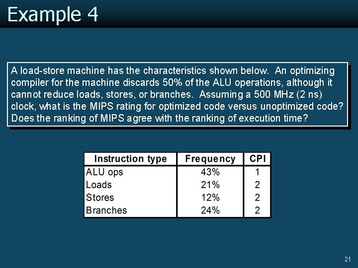
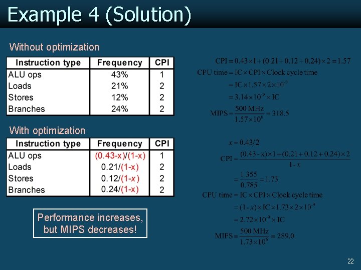
Example 4 A load-store machine has the characteristics shown below. An optimizing compiler for the machine discards 50% of the ALU operations, although it cannot reduce loads, stores, or branches. Assuming a 500 MHz (2 ns) clock, what is the MIPS rating for optimized code versus unoptimized code? Does the ranking of MIPS agree with the ranking of execution time? 21

Example 4 (Solution) Without optimization With optimization Performance increases, but MIPS decreases! 22

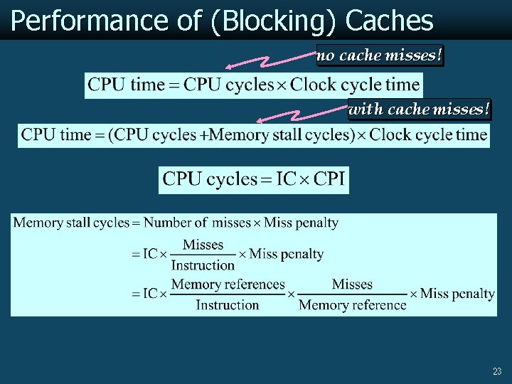
Performance of (Blocking) Caches no cache misses! with cache misses! 23

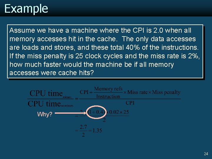
Example Assume we have a machine where the CPI is 2. 0 when all memory accesses hit in the cache. The only data accesses are loads and stores, and these total 40% of the instructions. If the miss penalty is 25 clock cycles and the miss rate is 2%, how much faster would the machine be if all memory accesses were cache hits? Why? 24

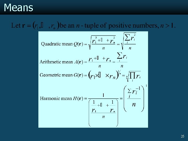
Means 25

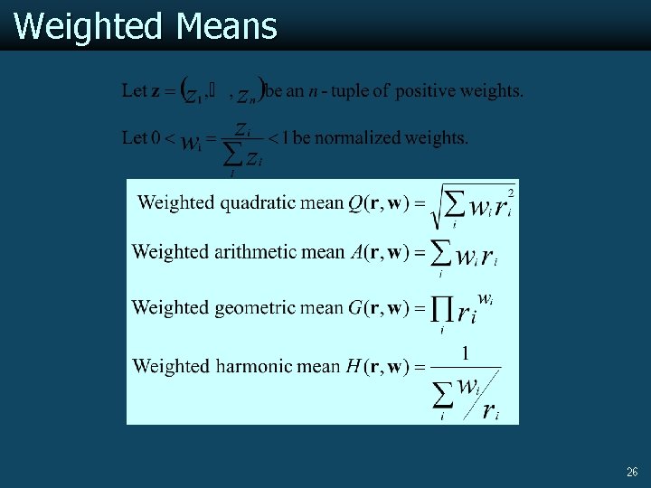
Weighted Means 26

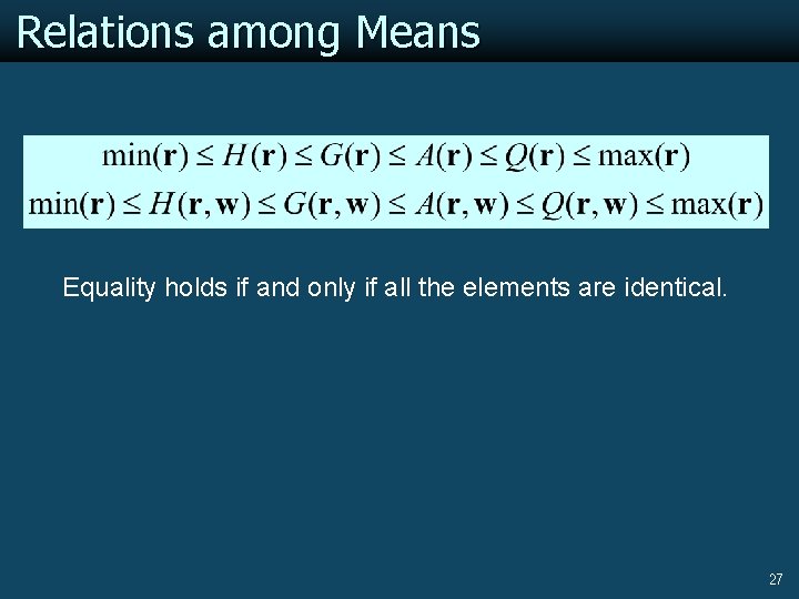
Relations among Means Equality holds if and only if all the elements are identical. 27

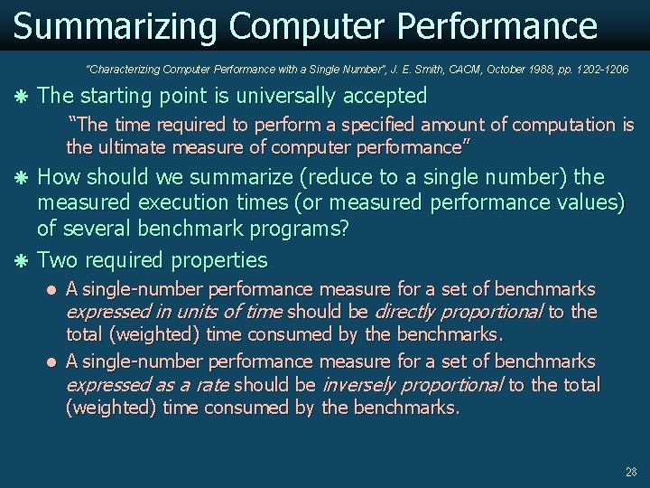
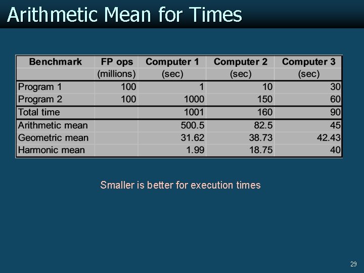
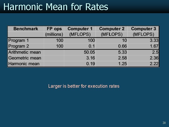
Summarizing Computer Performance “Characterizing Computer Performance with a Single Number”, J. E. Smith, CACM, October 1988, pp. 1202 -1206 ã The starting point is universally accepted “The time required to perform a specified amount of computation is the ultimate measure of computer performance” ã How should we summarize (reduce to a single number) the measured execution times (or measured performance values) of several benchmark programs? ã Two required properties l A single-number performance measure for a set of benchmarks expressed in units of time should be directly proportional to the total (weighted) time consumed by the benchmarks. l A single-number performance measure for a set of benchmarks expressed as a rate should be inversely proportional to the total (weighted) time consumed by the benchmarks. 28

Arithmetic Mean for Times Smaller is better for execution times 29

Harmonic Mean for Rates Larger is better for execution rates 30

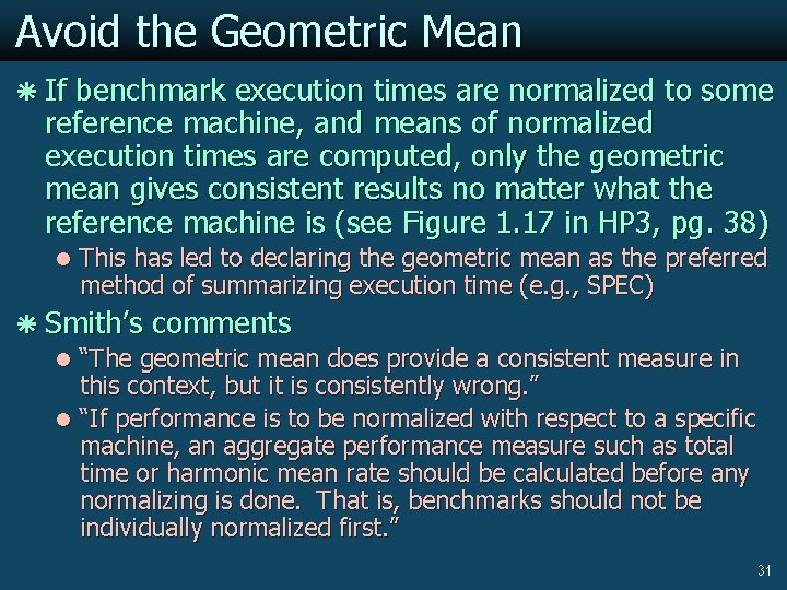
Avoid the Geometric Mean ã If benchmark execution times are normalized to some reference machine, and means of normalized execution times are computed, only the geometric mean gives consistent results no matter what the reference machine is (see Figure 1. 17 in HP 3, pg. 38) l This has led to declaring the geometric mean as the preferred method of summarizing execution time (e. g. , SPEC) ã Smith’s comments l “The geometric mean does provide a consistent measure in this context, but it is consistently wrong. ” l “If performance is to be normalized with respect to a specific machine, an aggregate performance measure such as total time or harmonic mean rate should be calculated before any normalizing is done. That is, benchmarks should not be individually normalized first. ” 31

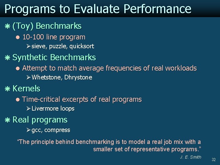
Programs to Evaluate Performance ã (Toy) Benchmarks l 10 -100 line program Ø sieve, puzzle, quicksort ã Synthetic Benchmarks l Attempt to match average frequencies of real workloads Ø Whetstone, Dhrystone ã Kernels l Time-critical excerpts of real programs Ø Livermore loops ã Real programs Ø gcc, compress “The principle behind benchmarking is to model a real job mix with a smaller set of representative programs. ” J. E. Smith 32

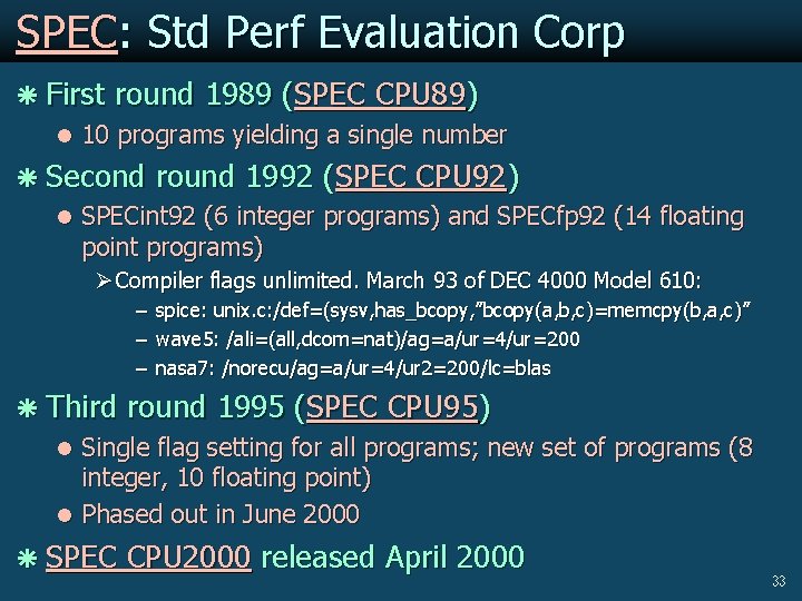
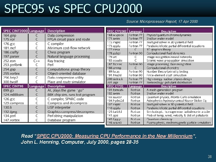
SPEC: Std Perf Evaluation Corp ã First round 1989 (SPEC CPU 89) l 10 programs yielding a single number ã Second round 1992 (SPEC CPU 92) l SPECint 92 (6 integer programs) and SPECfp 92 (14 floating point programs) Ø Compiler flags unlimited. March 93 of DEC 4000 Model 610: – – – spice: unix. c: /def=(sysv, has_bcopy, ”bcopy(a, b, c)=memcpy(b, a, c)” wave 5: /ali=(all, dcom=nat)/ag=a/ur=4/ur=200 nasa 7: /norecu/ag=a/ur=4/ur 2=200/lc=blas ã Third round 1995 (SPEC CPU 95) l Single flag setting for all programs; new set of programs (8 integer, 10 floating point) l Phased out in June 2000 ã SPEC CPU 2000 released April 2000 33

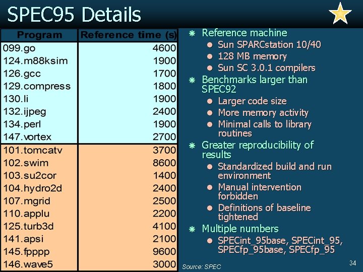
SPEC 95 Details ã Reference machine l Sun SPARCstation 10/40 l 128 MB memory l Sun SC 3. 0. 1 compilers ã Benchmarks larger than SPEC 92 l Larger code size l More memory activity l Minimal calls to library routines ã Greater reproducibility of results l Standardized build and run environment l Manual intervention forbidden l Definitions of baseline tightened ã Multiple numbers l SPECint_95 base, SPECint_95, SPECfp_95 base, SPECfp_95 Source: SPEC 34

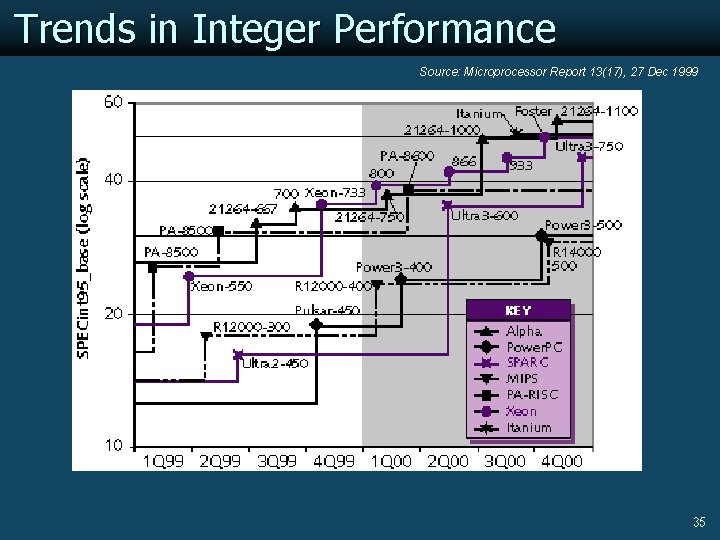
Trends in Integer Performance Source: Microprocessor Report 13(17), 27 Dec 1999 35

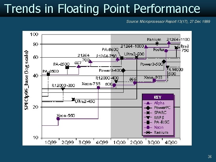
Trends in Floating Point Performance Source: Microprocessor Report 13(17), 27 Dec 1999 36

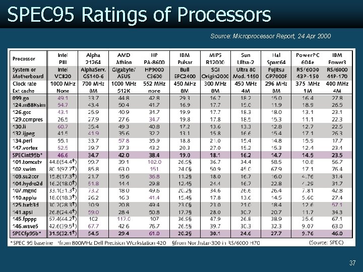
SPEC 95 Ratings of Processors Source: Microprocessor Report, 24 Apr 2000 37

SPEC 95 vs SPEC CPU 2000 Source: Microprocessor Report, 17 Apr 2000 Read “SPEC CPU 2000: Measuring CPU Performance in the New Millennium”, John L. Henning, Computer, July 2000, pages 28 -35 38

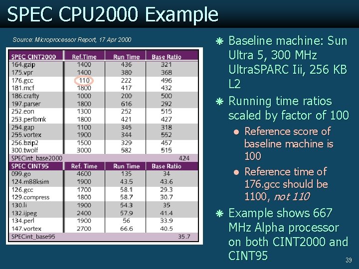
SPEC CPU 2000 Example Source: Microprocessor Report, 17 Apr 2000 ã Baseline machine: Sun Ultra 5, 300 MHz Ultra. SPARC Iii, 256 KB L 2 ã Running time ratios scaled by factor of 100 l Reference score of baseline machine is 100 l Reference time of 176. gcc should be 1100, not 110 ã Example shows 667 MHz Alpha processor on both CINT 2000 and CINT 95 39

Performance Evaluation ã Given sales is a function of performance relative to the competition, big investment in improving product as reported by performance summary ã Good products created when you have: l Good benchmarks l Good ways to summarize performance ã If benchmarks/summary inadequate, then choose between improving product for real programs vs. improving product to get more sales l Sales almost always wins! ã Execution time is the measure of computer performance! ã What about cost? 40

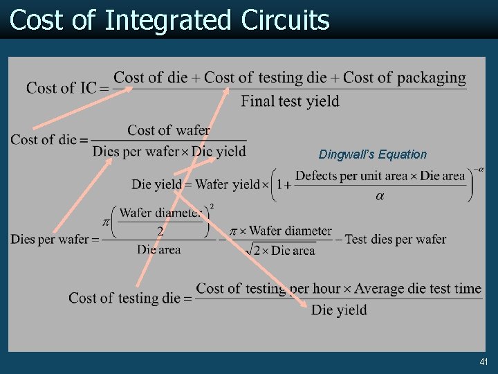
Cost of Integrated Circuits Dingwall’s Equation 41

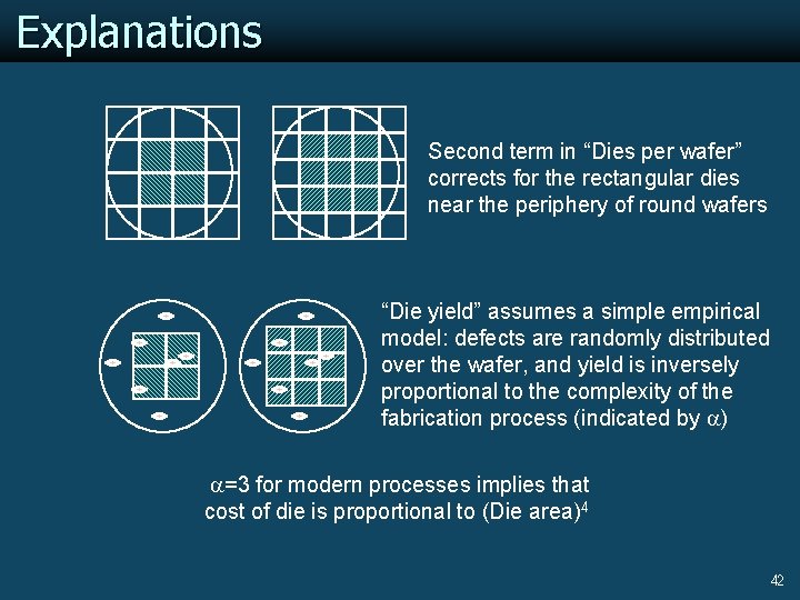
Explanations Second term in “Dies per wafer” corrects for the rectangular dies near the periphery of round wafers “Die yield” assumes a simple empirical model: defects are randomly distributed over the wafer, and yield is inversely proportional to the complexity of the fabrication process (indicated by a) a=3 for modern processes implies that cost of die is proportional to (Die area)4 42

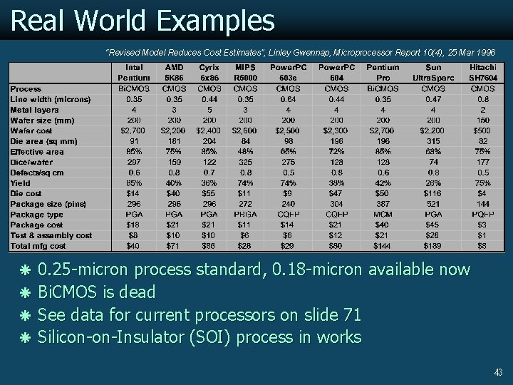
Real World Examples “Revised Model Reduces Cost Estimates”, Linley Gwennap, Microprocessor Report 10(4), 25 Mar 1996 ã 0. 25 -micron process standard, 0. 18 -micron available now ã Bi. CMOS is dead ã See data for current processors on slide 71 ã Silicon-on-Insulator (SOI) process in works 43

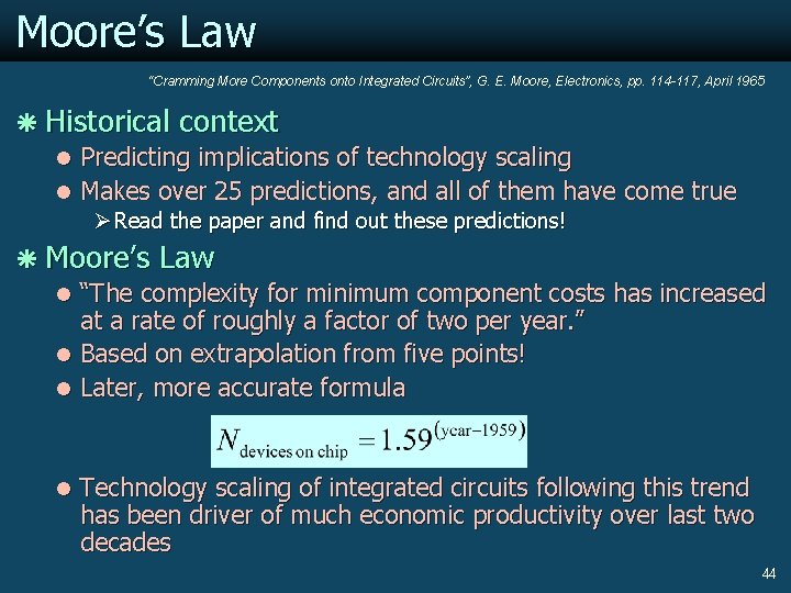
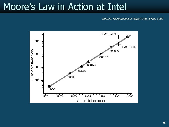
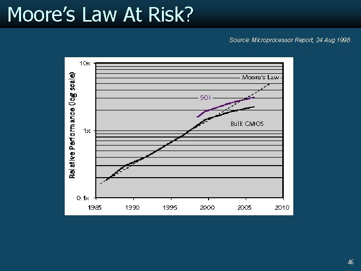
Moore’s Law “Cramming More Components onto Integrated Circuits”, G. E. Moore, Electronics, pp. 114 -117, April 1965 ã Historical context l Predicting implications of technology scaling l Makes over 25 predictions, and all of them have come true Ø Read the paper and find out these predictions! ã Moore’s Law l “The complexity for minimum component costs has increased at a rate of roughly a factor of two per year. ” l Based on extrapolation from five points! l Later, more accurate formula l Technology scaling of integrated circuits following this trend has been driver of much economic productivity over last two decades 44

Moore’s Law in Action at Intel Source: Microprocessor Report 9(6), 8 May 1995 45

Moore’s Law At Risk? Source: Microprocessor Report, 24 Aug 1998 46

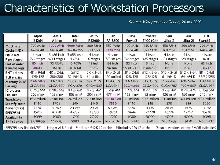
Characteristics of Workstation Processors Source: Microprocessor Report, 24 Apr 2000 47

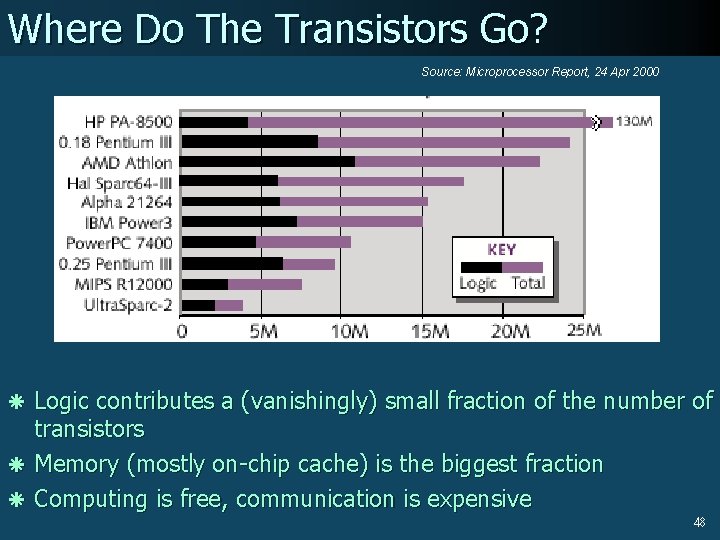
Where Do The Transistors Go? Source: Microprocessor Report, 24 Apr 2000 ã Logic contributes a (vanishingly) small fraction of the number of transistors ã Memory (mostly on-chip cache) is the biggest fraction ã Computing is free, communication is expensive 48

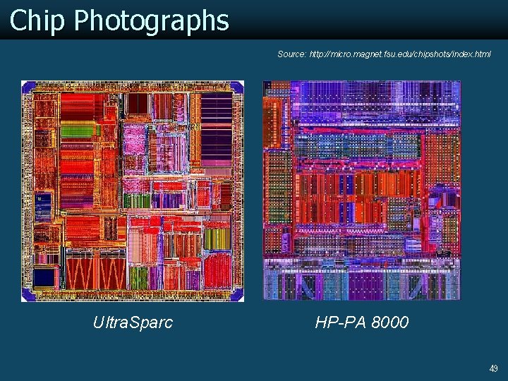
Chip Photographs Source: http: //micro. magnet. fsu. edu/chipshots/index. html Ultra. Sparc HP-PA 8000 49

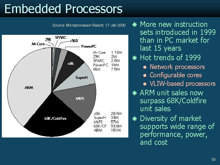
Embedded Processors Source: Microprocessor Report, 17 Jan 2000 ã More new instruction sets introduced in 1999 than in PC market for last 15 years ã Hot trends of 1999 l Network processors l Configurable cores l VLIW-based processors ã ARM unit sales now surpass 68 K/Coldfire unit sales ã Diversity of market supports wide range of performance, power, and cost 50

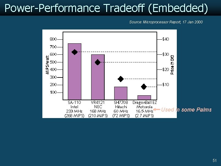
Power-Performance Tradeoff (Embedded) Source: Microprocessor Report, 17 Jan 2000 Used in some Palms 51