Chapter 6 Random Error in Chemical Analyses 6

Chapter 6 Random Error in Chemical Analyses

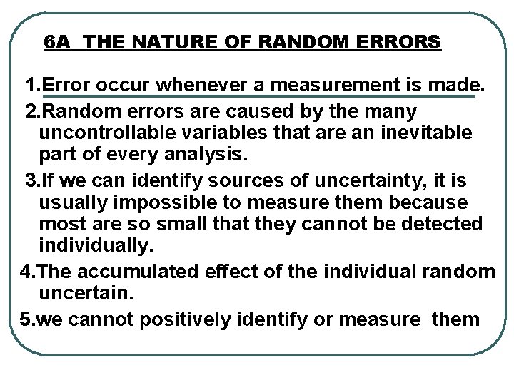
6 A THE NATURE OF RANDOM ERRORS 1. Error occur whenever a measurement is made. 2. Random errors are caused by the many uncontrollable variables that are an inevitable part of every analysis. 3. If we can identify sources of uncertainty, it is usually impossible to measure them because most are so small that they cannot be detected individually. 4. The accumulated effect of the individual random uncertain. 5. we cannot positively identify or measure them

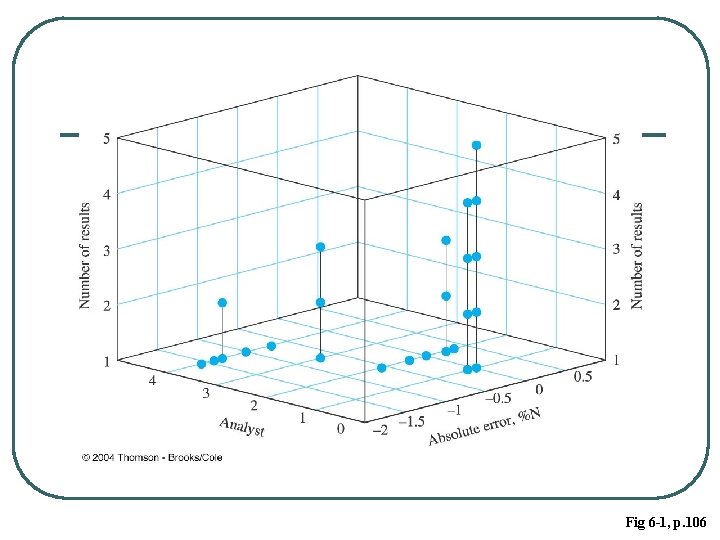
Fig 6 -1, p. 106

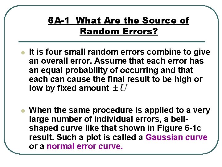
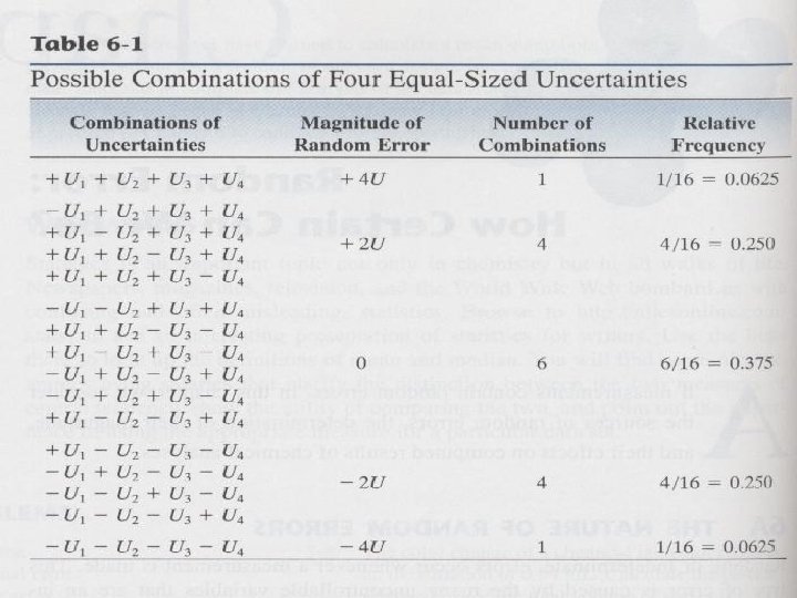
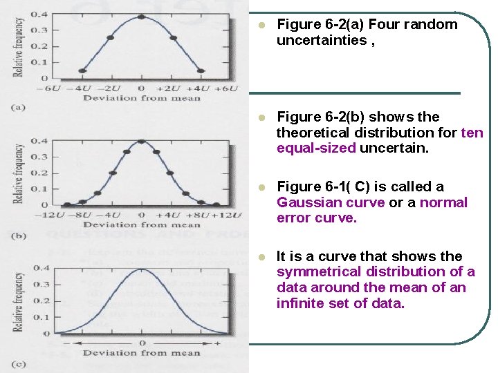
6 A-1 What Are the Source of Random Errors? l It is four small random errors combine to give an overall error. Assume that each error has an equal probability of occurring and that each can cause the final result to be high or low by fixed amount l When the same procedure is applied to a very large number of individual errors, a bellshaped curve like that shown in Figure 6 -1 c result. Such a plot is called a Gaussian curve or a normal error curve.

l Figure 6 -2(a) Four random uncertainties , l Figure 6 -2(b) shows theoretical distribution for ten equal-sized uncertain. l Figure 6 -1( C) is called a Gaussian curve or a normal error curve. l It is a curve that shows the symmetrical distribution of a data around the mean of an infinite set of data.

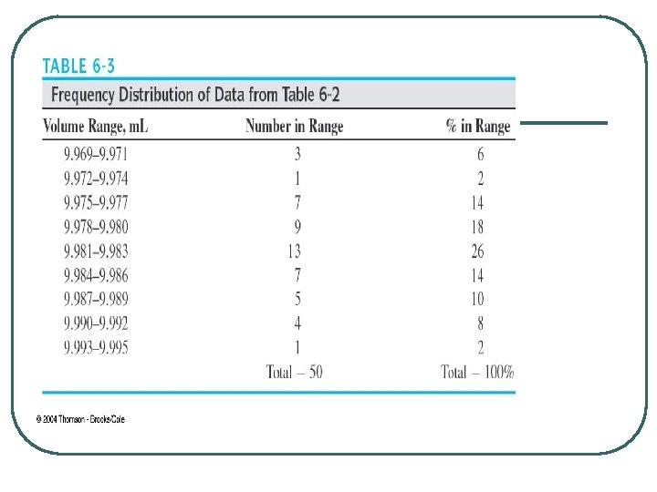
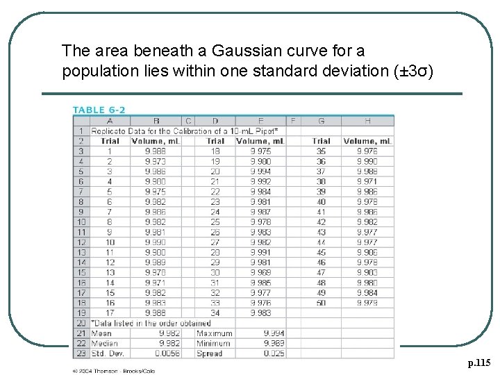
6 A-2 Describing the Distribution Of Experimental Data l Table 6 -2 are typical of those obtained by an worker weighing to the nearest milligram (which correspond to 0. 001 m. L) on a top loading balance and making every effort to avoid systematic error.

Table 6 -2, p. 108

Table 6 -3, p. 108

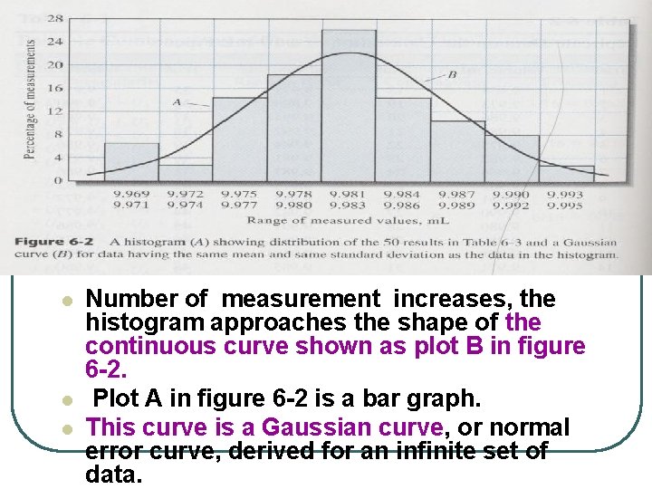
l l l Number of measurement increases, the histogram approaches the shape of the continuous curve shown as plot B in figure 6 -2. Plot A in figure 6 -2 is a bar graph. This curve is a Gaussian curve, or normal error curve, derived for an infinite set of data.

6 B TREATING RANDOM ERRORS WITH STATISTICS? 1. Statistical methods to evaluate the random errors discussed in the preceding section, we base statistic analyses on assumption that random errors in analytical results follow a Gaussian, 2. Statistics only reveal information that is already present in a data set. No new information is created by statistical treatments. Statistical analysis can look at our data in different ways and make objective and intelligent decisions regarding their quality and use.

6 B-1 Sample and Populations 1. We infer information about a population or universe from observations made on a subset or sample. 2. The population is the collection all measurements of interest and must be carefully defined by the experimenter. It is finite and real. （conceptual） 3. Statistical laws have been derived for populations , often they must be modified substantially when applied to a small sample because a few data points may not represent the entire population. 4. Do not confuse the statistical sample with the analytical sample. Four analytical samples analyzed in the laboratory represent a single statistical sample.

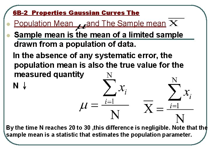
6 B-2 Properties Gaussian Curves The Population Mean and The Sample mean l Sample mean is the mean of a limited sample drawn from a population of data. In the absence of any systematic error, the population mean is also the true value for the measured quantity N↓ l By the time N reaches 20 to 30 , this difference is negligible. Note that the sample mean is a statistic that estimates the population parameter.

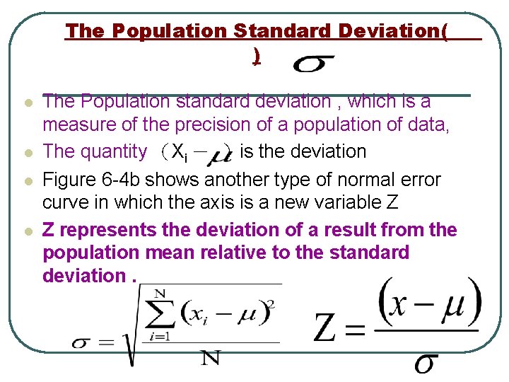
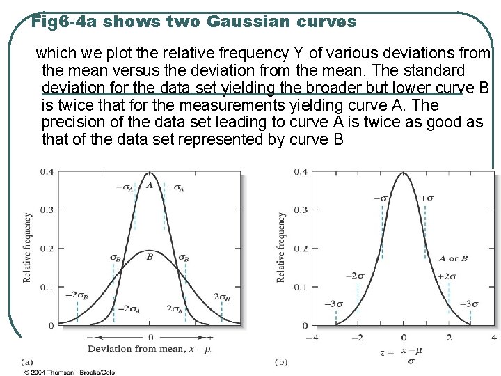
The Population Standard Deviation( ) l l The Population standard deviation , which is a measure of the precision of a population of data, The quantity （Xi － ）is the deviation Figure 6 -4 b shows another type of normal error curve in which the axis is a new variable Z Z represents the deviation of a result from the population mean relative to the standard deviation.

Fig 6 -4 a shows two Gaussian curves which we plot the relative frequency Y of various deviations from the mean versus the deviation from the mean. The standard deviation for the data set yielding the broader but lower curve B is twice that for the measurements yielding curve A. The precision of the data set leading to curve A is twice as good as that of the data set represented by curve B

Normal error curve has several general properties 1、The mean occurs at the central point of maximum frequency. 2、There is a symmetrical distribution of positive and negative about the maximum, 3、There is an exponential decrease in frequency as the magnitude of the deviations increases. Thus, small uncertainties are observed much more often than very large ones.

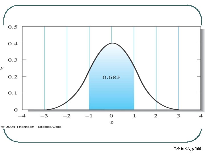
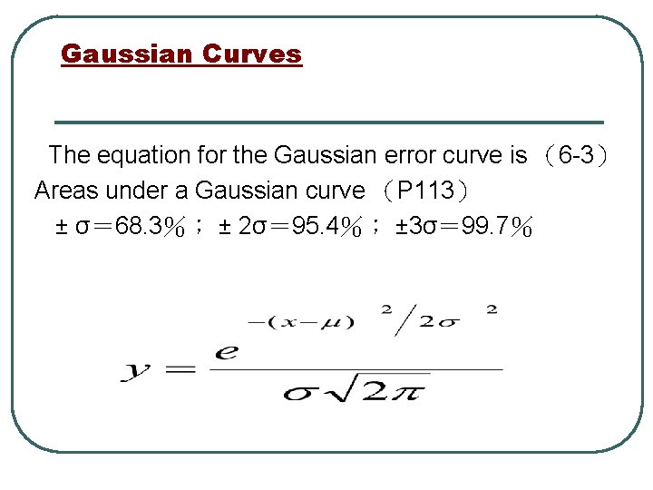
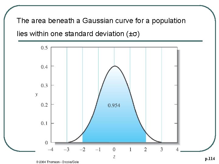
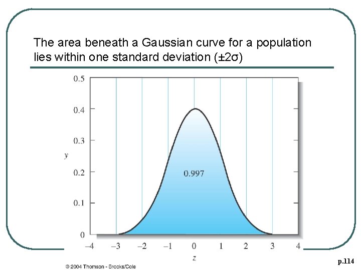
Gaussian Curves The equation for the Gaussian error curve is （6 -3） Areas under a Gaussian curve （P 113） ± σ＝ 68. 3％； ± 2σ＝ 95. 4％； ± 3σ＝ 99. 7％

The area beneath a Gaussian curve for a population lies within one standard deviation (±σ) p. 114

The area beneath a Gaussian curve for a population lies within one standard deviation (± 2σ) p. 114

The area beneath a Gaussian curve for a population lies within one standard deviation (± 3σ) p. 115

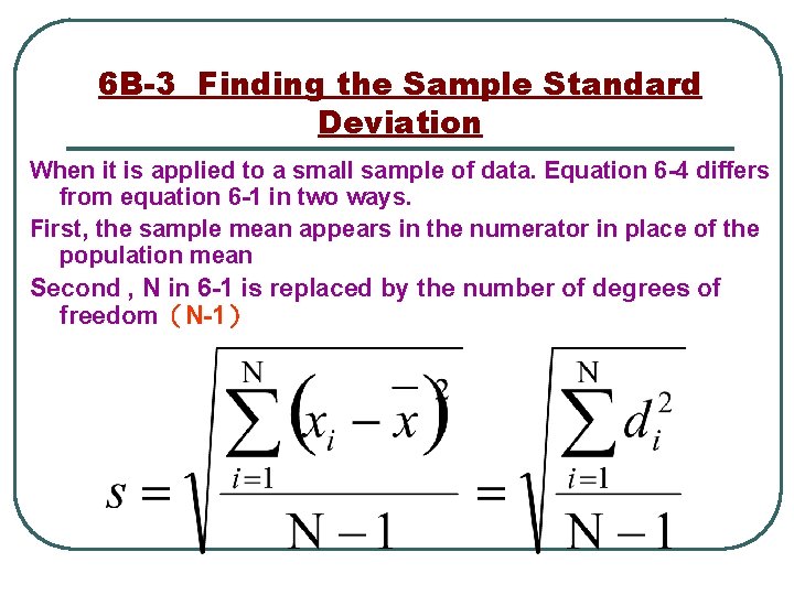
6 B-3 Finding the Sample Standard Deviation When it is applied to a small sample of data. Equation 6 -4 differs from equation 6 -1 in two ways. First, the sample mean appears in the numerator in place of the population mean Second , N in 6 -1 is replaced by the number of degrees of freedom（N-1）

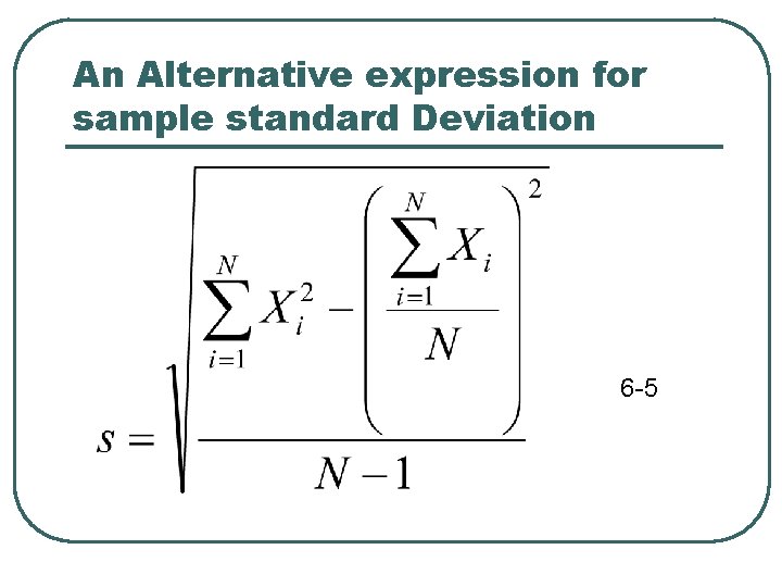
An Alternative expression for sample standard Deviation 6 -5

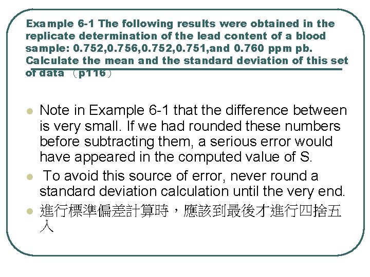
Example 6 -1 The following results were obtained in the replicate determination of the lead content of a blood sample: 0. 752, 0. 756, 0. 752, 0. 751, and 0. 760 ppm pb. Calculate the mean and the standard deviation of this set of data （p 116） l l l Note in Example 6 -1 that the difference between is very small. If we had rounded these numbers before subtracting them, a serious error would have appeared in the computed value of S. To avoid this source of error, never round a standard deviation calculation until the very end. 進行標準偏差計算時，應該到最後才進行四捨五 入

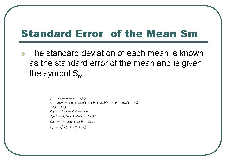
Standard Error of the Mean Sm l The standard deviation of each mean is known as the standard error of the mean and is given the symbol Sm

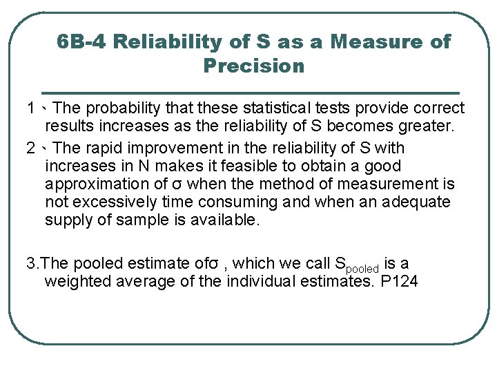
6 B-4 Reliability of S as a Measure of Precision 1、The probability that these statistical tests provide correct results increases as the reliability of S becomes greater. 2、The rapid improvement in the reliability of S with increases in N makes it feasible to obtain a good approximation of σ when the method of measurement is not excessively time consuming and when an adequate supply of sample is available. 3. The pooled estimate ofσ , which we call Spooled is a weighted average of the individual estimates. P 124

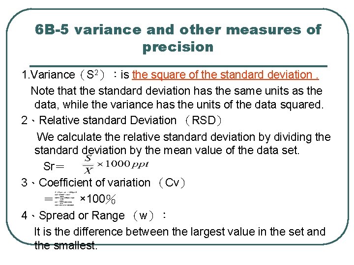
6 B-5 variance and other measures of precision 1. Variance（S 2）：is the square of the standard deviation. Note that the standard deviation has the same units as the data, while the variance has the units of the data squared. 2、Relative standard Deviation （RSD） We calculate the relative standard deviation by dividing the standard deviation by the mean value of the data set. Sr＝ 3、Coefficient of variation （Cv） ＝ × 100％ 4、Spread or Range （w）： It is the difference between the largest value in the set and the smallest.

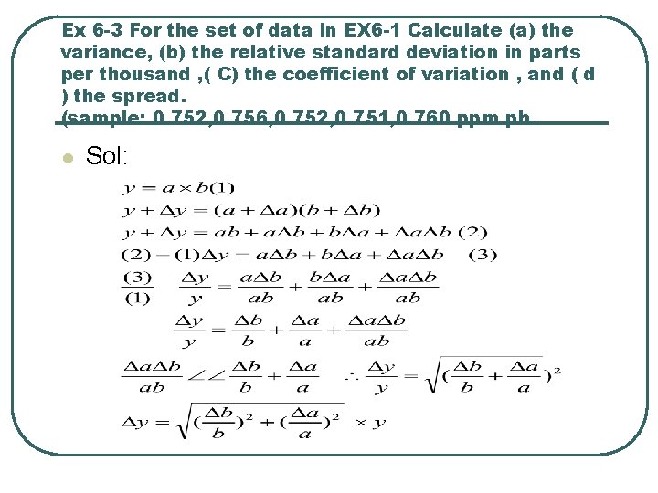
Ex 6 -3 For the set of data in EX 6 -1 Calculate (a) the variance, (b) the relative standard deviation in parts per thousand , ( C) the coefficient of variation , and ( d ) the spread. (sample: 0. 752, 0. 756, 0. 752, 0. 751, 0. 760 ppm pb. l Sol:

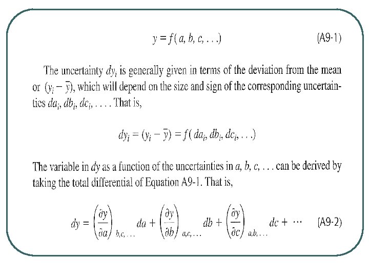
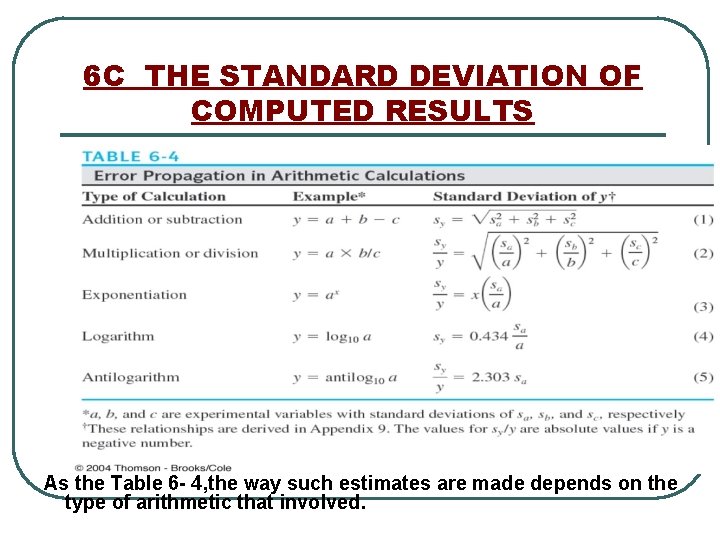
6 C THE STANDARD DEVIATION OF COMPUTED RESULTS As the Table 6 - 4, the way such estimates are made depends on the type of arithmetic that involved.

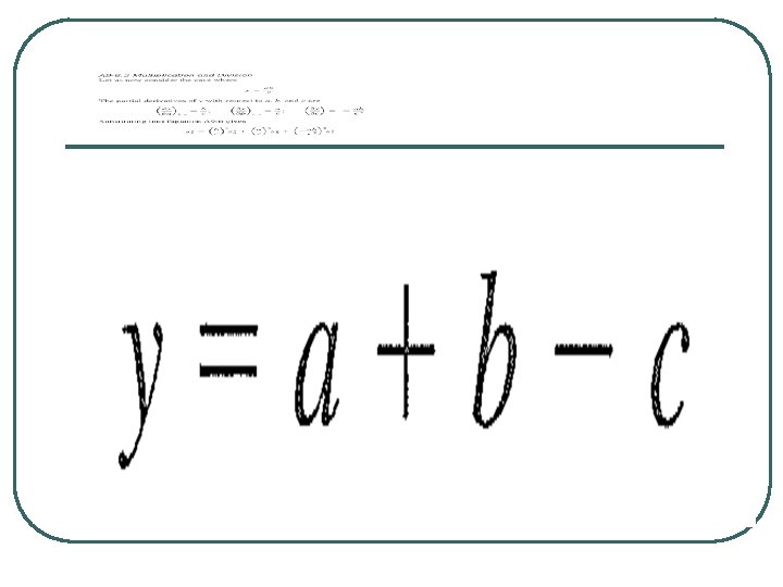
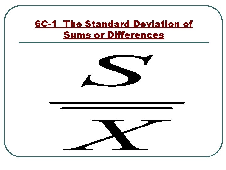
6 C-1 The Standard Deviation of Sums or Differences

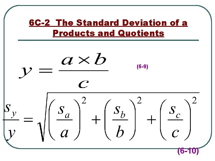
6 C-2 The Standard Deviation of a Products and Quotients (6 -9) (6 -10)

6 D REPORTING COMPUTED DATA l The significant figure in a number are all the certain digits plus the first uncertain digit.

6 D-1 The Significant Figure Convention l l Express data in scientific notation to avoid confusion in determining whether terminal zeros are significant. Rules for determining the number of significant figures: 1. Disregard all initial zeros. 2. Disregard all final zeros unless they follow a decimal point. 3. All remaining digits including zeros between nonzero digits are significant

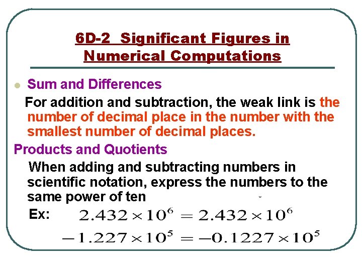
6 D-2 Significant Figures in Numerical Computations Sum and Differences For addition and subtraction, the weak link is the number of decimal place in the number with the smallest number of decimal places. Products and Quotients When adding and subtracting numbers in scientific notation, express the numbers to the same power of ten Ex: l

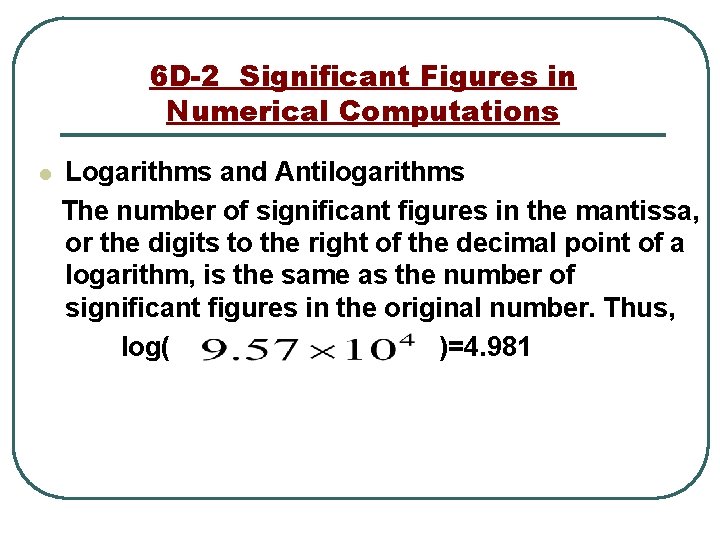
6 D-2 Significant Figures in Numerical Computations l Logarithms and Antilogarithms The number of significant figures in the mantissa, or the digits to the right of the decimal point of a logarithm, is the same as the number of significant figures in the original number. Thus, log( )=4. 981

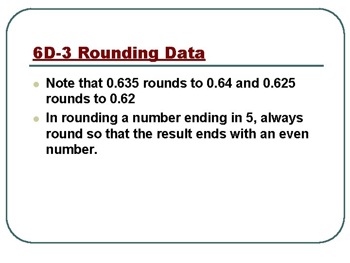
6 D-3 Rounding Data l l Note that 0. 635 rounds to 0. 64 and 0. 625 rounds to 0. 62 In rounding a number ending in 5, always round so that the result ends with an even number.

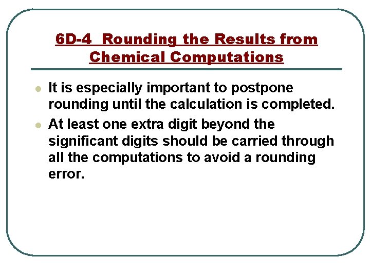
6 D-4 Rounding the Results from Chemical Computations l l It is especially important to postpone rounding until the calculation is completed. At least one extra digit beyond the significant digits should be carried through all the computations to avoid a rounding error.

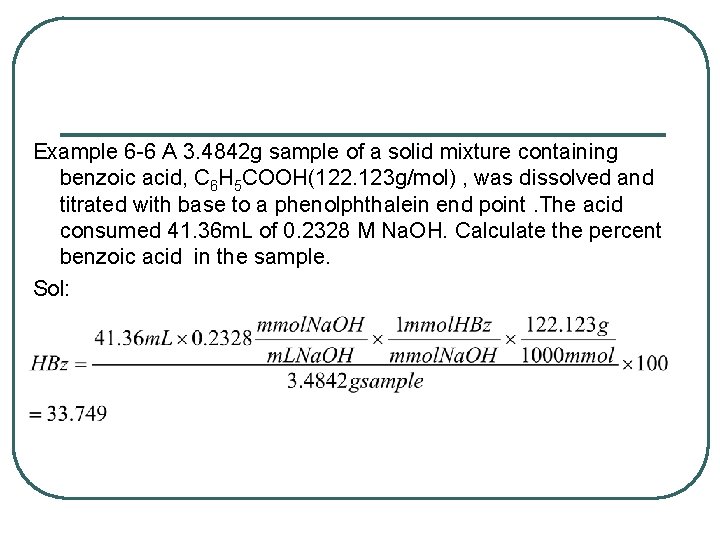
Example 6 -6 A 3. 4842 g sample of a solid mixture containing benzoic acid, C 6 H 5 COOH(122. 123 g/mol) , was dissolved and titrated with base to a phenolphthalein end point. The acid consumed 41. 36 m. L of 0. 2328 M Na. OH. Calculate the percent benzoic acid in the sample. Sol: