Chapter 3 Data and Signals Hanyang University Prof

Chapter 3 Data and Signals Hanyang University Prof. Inwhee Joe 3. 1

Note To be transmitted, data must be transformed to electromagnetic signals. 3. 2

3 -1 ANALOG AND DIGITAL Data can be analog or digital. The term analog data refers to information that is continuous; digital data refers to information that has discrete states. Analog data take on continuous values. Digital data take on discrete values. Topics discussed in this section: Analog and Digital Data Analog and Digital Signals Periodic and Nonperiodic Signals 3. 3

Note Data can be analog or digital. Analog data are continuous and take continuous values. Digital data have discrete states and take discrete values. 3. 4

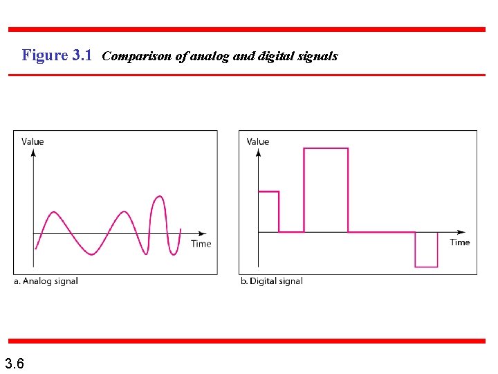
Note Signals can be analog or digital. Analog signals can have an infinite number of values in a range; digital signals can have only a limited number of values. 3. 5

Figure 3. 1 Comparison of analog and digital signals 3. 6

Note In data communications, we commonly use periodic analog signals and nonperiodic digital signals. 3. 7

3 -2 PERIODIC ANALOG SIGNALS Periodic analog signals can be classified as simple or composite. A simple periodic analog signal, a sine wave, cannot be decomposed into simpler signals. A composite periodic analog signal is composed of multiple sine waves. Topics discussed in this section: Sine Wavelength Time and Frequency Domain Composite Signals Bandwidth 3. 8

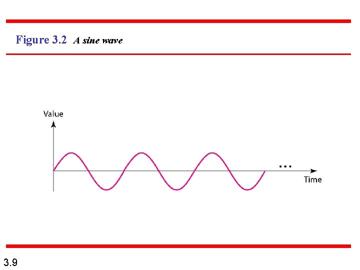
Figure 3. 2 A sine wave 3. 9

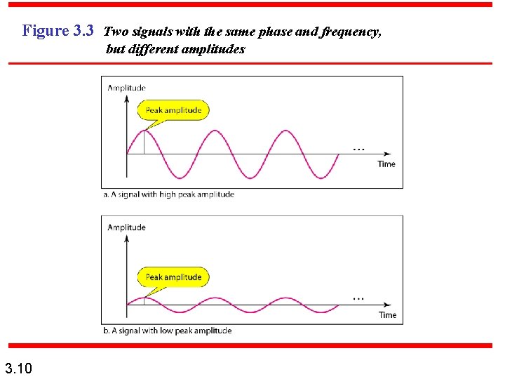
Figure 3. 3 Two signals with the same phase and frequency, but different amplitudes 3. 10

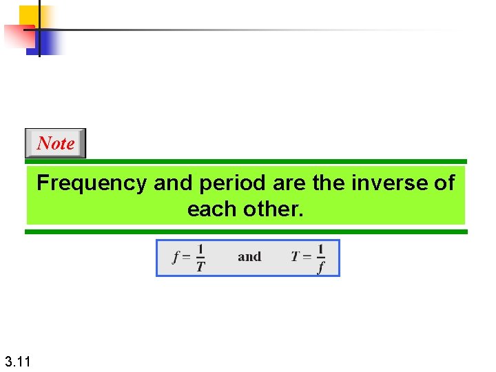
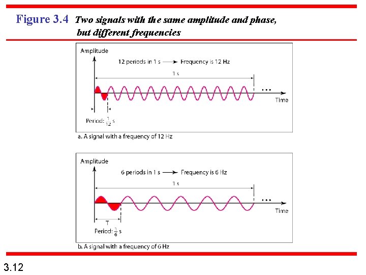
Note Frequency and period are the inverse of each other. 3. 11

Figure 3. 4 Two signals with the same amplitude and phase, but different frequencies 3. 12

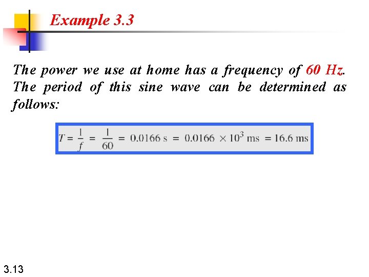
Example 3. 3 The power we use at home has a frequency of 60 Hz. The period of this sine wave can be determined as follows: 3. 13

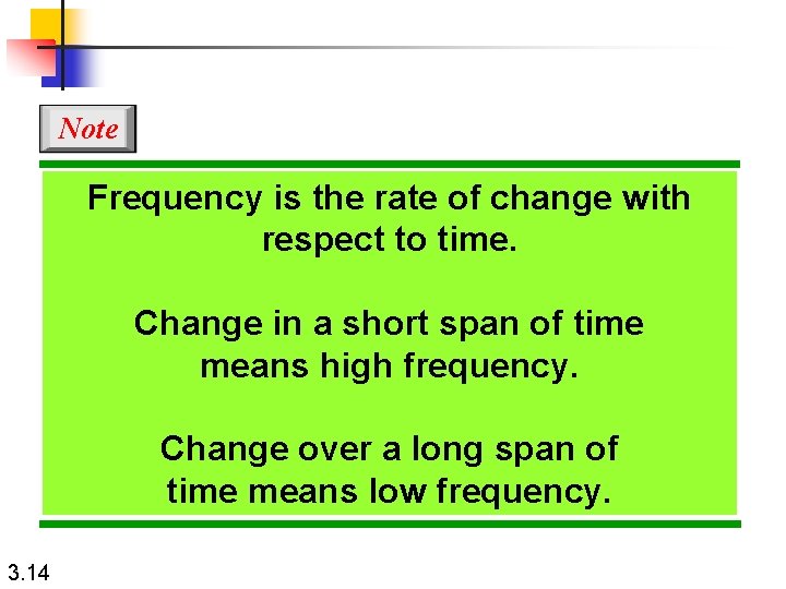
Note Frequency is the rate of change with respect to time. Change in a short span of time means high frequency. Change over a long span of time means low frequency. 3. 14

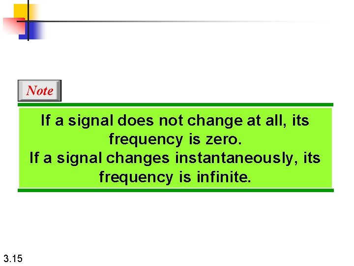
Note If a signal does not change at all, its frequency is zero. If a signal changes instantaneously, its frequency is infinite. 3. 15

Note Phase describes the position of the waveform relative to time 0. 3. 16

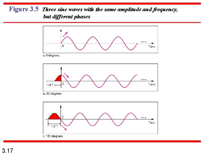
Figure 3. 5 Three sine waves with the same amplitude and frequency, but different phases 3. 17

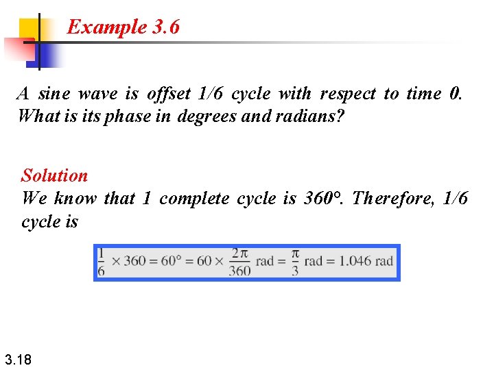
Example 3. 6 A sine wave is offset 1/6 cycle with respect to time 0. What is its phase in degrees and radians? Solution We know that 1 complete cycle is 360°. Therefore, 1/6 cycle is 3. 18

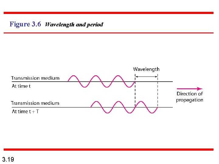
Figure 3. 6 Wavelength and period 3. 19

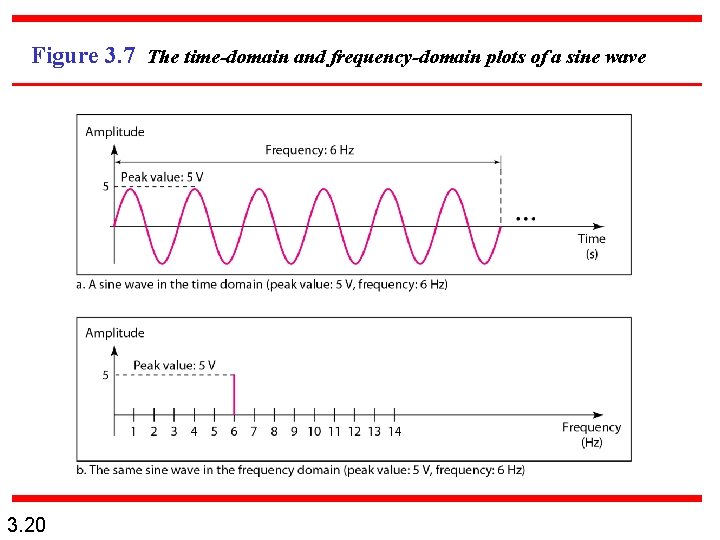
Figure 3. 7 The time-domain and frequency-domain plots of a sine wave 3. 20

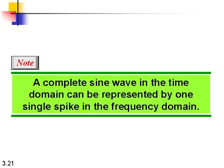
Note A complete sine wave in the time domain can be represented by one single spike in the frequency domain. 3. 21

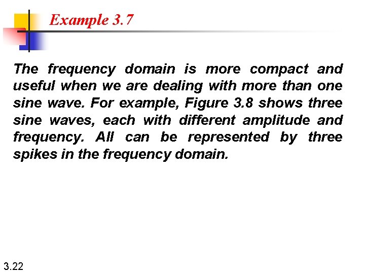
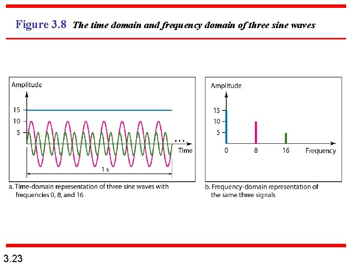
Example 3. 7 The frequency domain is more compact and useful when we are dealing with more than one sine wave. For example, Figure 3. 8 shows three sine waves, each with different amplitude and frequency. All can be represented by three spikes in the frequency domain. 3. 22

Figure 3. 8 The time domain and frequency domain of three sine waves 3. 23

Note A single-frequency sine wave is not useful in data communications; we need to send a composite signal, a signal made of many simple sine waves. 3. 24

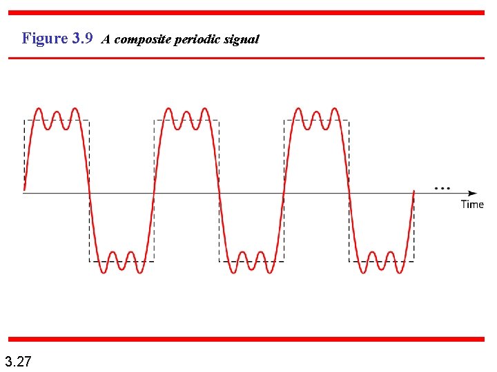
Note According to Fourier analysis, any composite signal is a combination of simple sine waves with different frequencies, amplitudes, and phases. Fourier analysis is discussed in Appendix C. 3. 25

Note If the composite signal is periodic, the decomposition gives a series of signals with discrete frequencies; if the composite signal is nonperiodic, the decomposition gives a combination of sine waves with continuous frequencies. 3. 26

Figure 3. 9 A composite periodic signal 3. 27

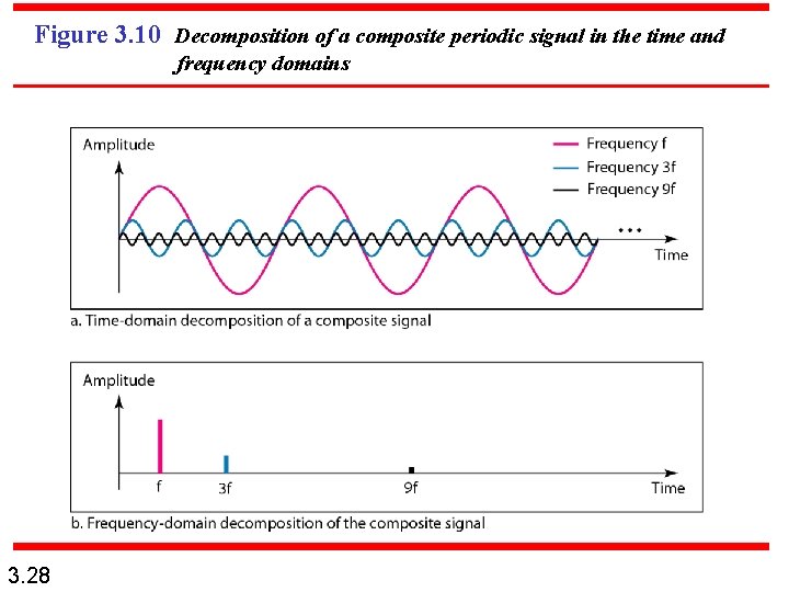
Figure 3. 10 Decomposition of a composite periodic signal in the time and frequency domains 3. 28

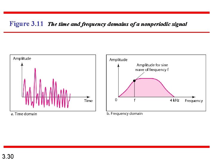
Example 3. 9 Figure 3. 11 shows a nonperiodic composite signal. It can be the signal created by a microphone or a telephone set when a word or two is pronounced. In this case, the composite signal cannot be periodic, because that implies that we are repeating the same word or words with exactly the same tone. 3. 29

Figure 3. 11 The time and frequency domains of a nonperiodic signal 3. 30

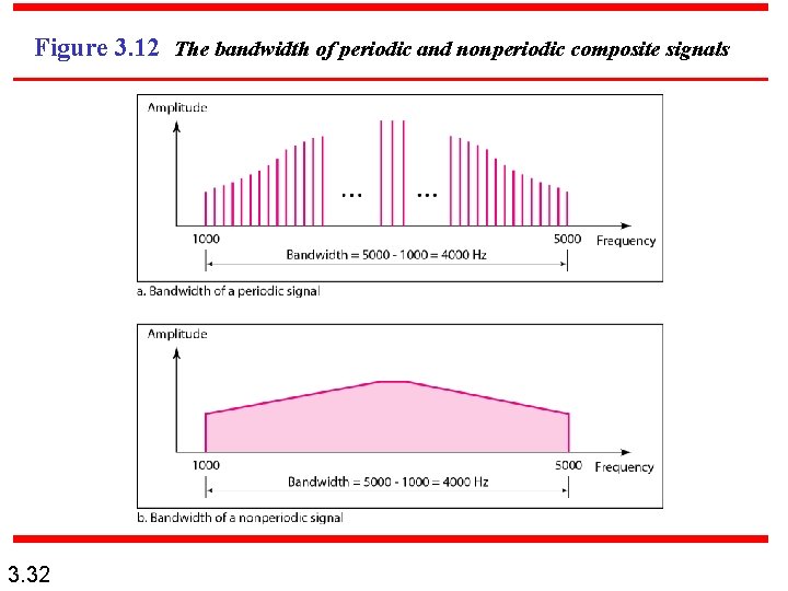
Note The bandwidth of a composite signal is the difference between the highest and the lowest frequencies contained in that signal. 3. 31

Figure 3. 12 The bandwidth of periodic and nonperiodic composite signals 3. 32

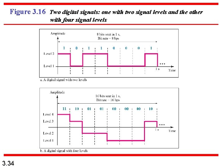
3 -3 DIGITAL SIGNALS In addition to being represented by an analog signal, information can also be represented by a digital signal. For example, a 1 can be encoded as a positive voltage and a 0 as zero voltage. A digital signal can have more than two levels. In this case, we can send more than 1 bit for each level. Topics discussed in this section: Bit Rate Bit Length Digital Signal as a Composite Analog Signal Application Layer 3. 33

Figure 3. 16 Two digital signals: one with two signal levels and the other with four signal levels 3. 34

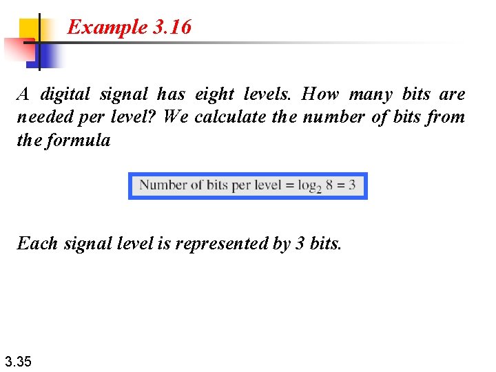
Example 3. 16 A digital signal has eight levels. How many bits are needed per level? We calculate the number of bits from the formula Each signal level is represented by 3 bits. 3. 35

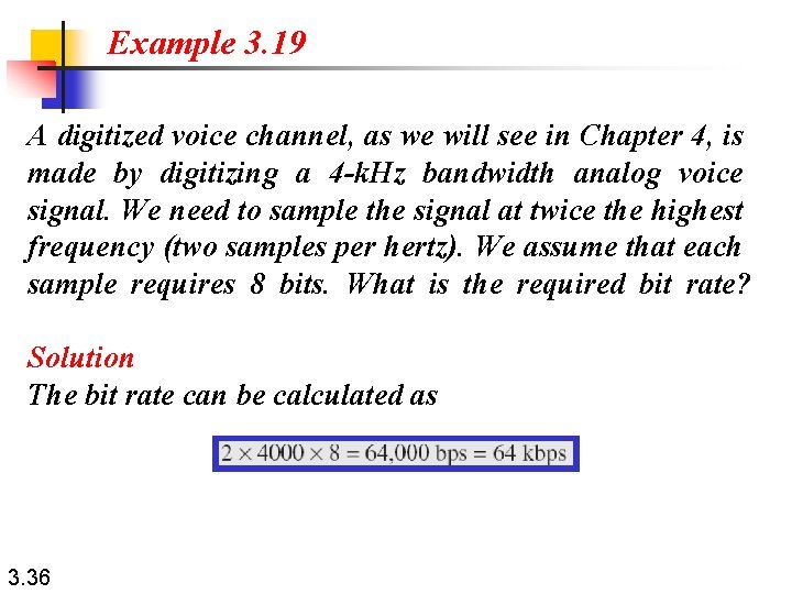
Example 3. 19 A digitized voice channel, as we will see in Chapter 4, is made by digitizing a 4 -k. Hz bandwidth analog voice signal. We need to sample the signal at twice the highest frequency (two samples per hertz). We assume that each sample requires 8 bits. What is the required bit rate? Solution The bit rate can be calculated as 3. 36

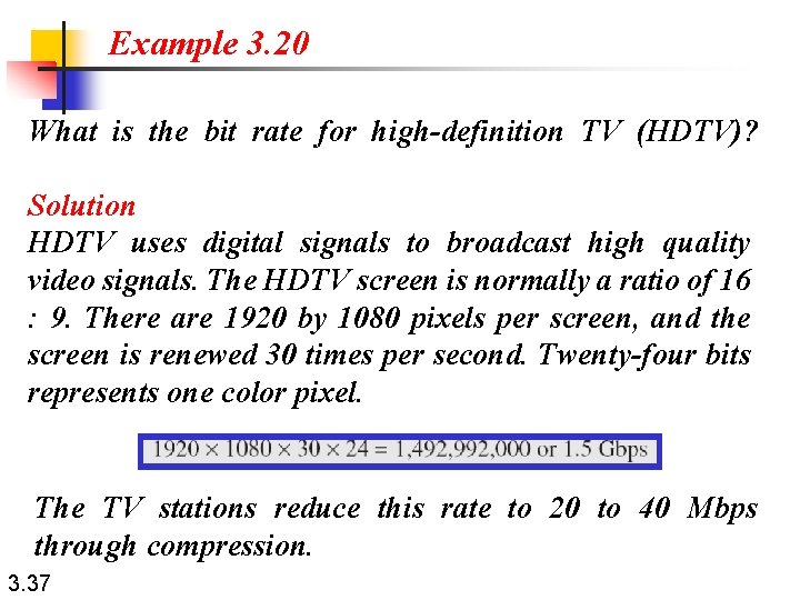
Example 3. 20 What is the bit rate for high-definition TV (HDTV)? Solution HDTV uses digital signals to broadcast high quality video signals. The HDTV screen is normally a ratio of 16 : 9. There are 1920 by 1080 pixels per screen, and the screen is renewed 30 times per second. Twenty-four bits represents one color pixel. The TV stations reduce this rate to 20 to 40 Mbps through compression. 3. 37

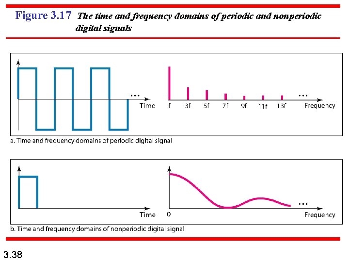
Figure 3. 17 The time and frequency domains of periodic and nonperiodic digital signals 3. 38

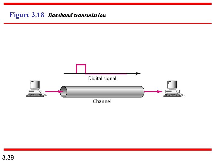
Figure 3. 18 Baseband transmission 3. 39

Note A digital signal is a composite analog signal with an infinite bandwidth. 3. 40

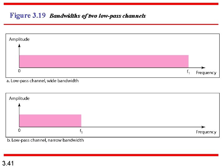
Figure 3. 19 Bandwidths of two low-pass channels 3. 41

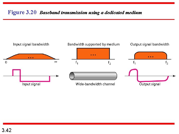
Figure 3. 20 Baseband transmission using a dedicated medium 3. 42

Note Baseband transmission of a digital signal that preserves the shape of the digital signal is possible only if we have a low-pass channel with an infinite or very wide bandwidth. 3. 43

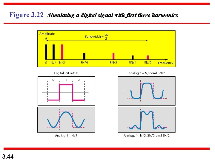
Figure 3. 22 Simulating a digital signal with first three harmonics 3. 44

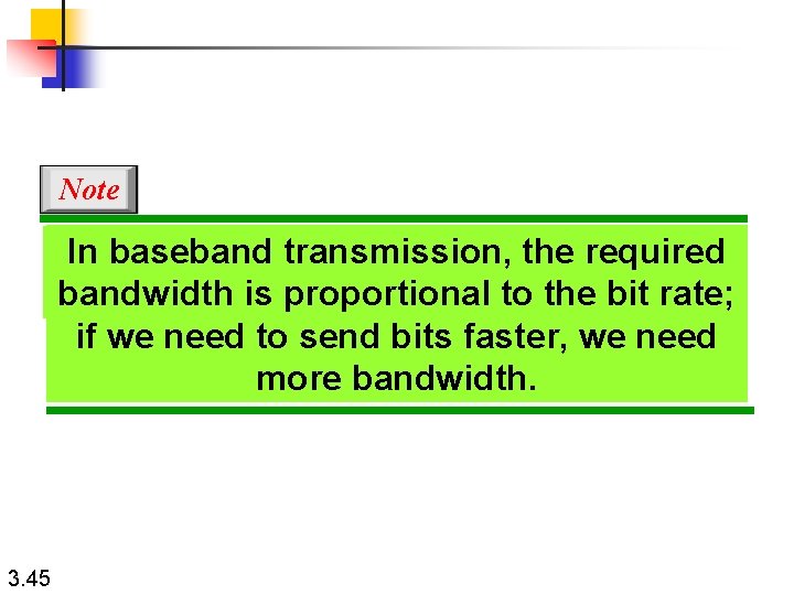
Note In baseband transmission, the required bandwidth is In baseband transmission, the required proportional to the bit rate; if we need to send bits faster, we needto more bandwidth is proportional thebandwidth. bit rate; if we need to send bits faster, we need more bandwidth. 3. 45

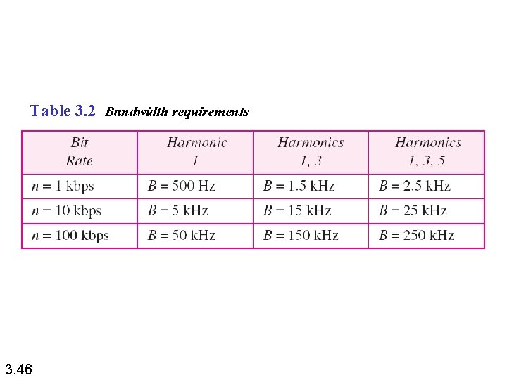
Table 3. 2 Bandwidth requirements 3. 46

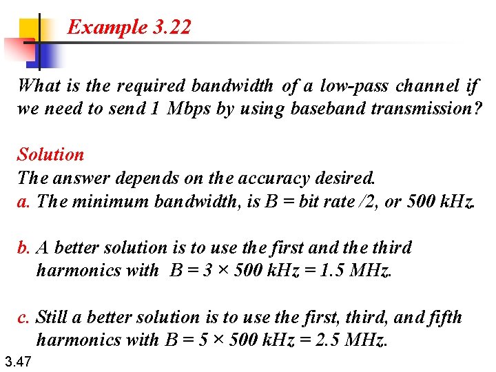
Example 3. 22 What is the required bandwidth of a low-pass channel if we need to send 1 Mbps by using baseband transmission? Solution The answer depends on the accuracy desired. a. The minimum bandwidth, is B = bit rate /2, or 500 k. Hz. b. A better solution is to use the first and the third harmonics with B = 3 × 500 k. Hz = 1. 5 MHz. c. Still a better solution is to use the first, third, and fifth harmonics with B = 5 × 500 k. Hz = 2. 5 MHz. 3. 47

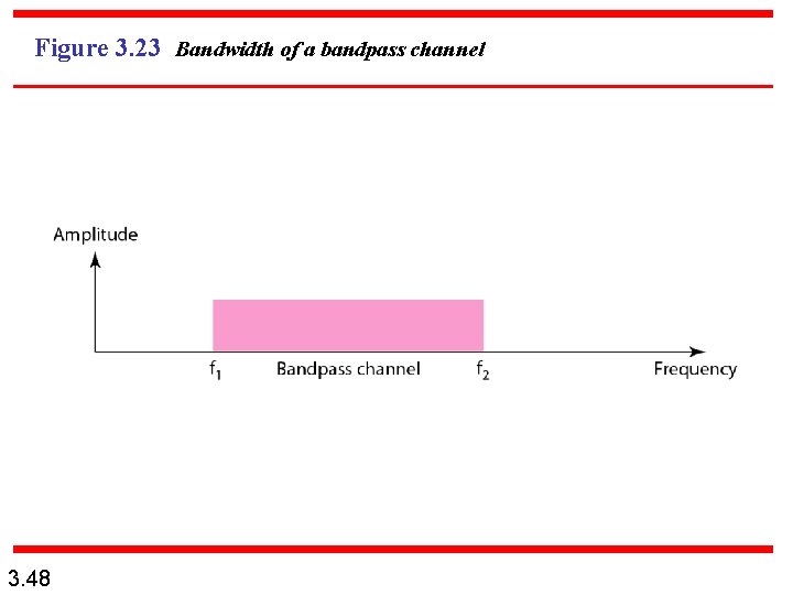
Figure 3. 23 Bandwidth of a bandpass channel 3. 48

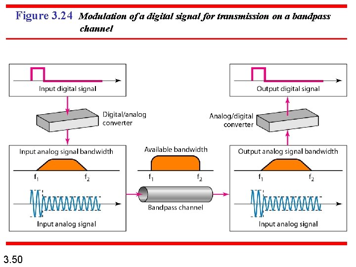
Note If the available channel is a bandpass channel, we cannot send the digital signal directly to the channel; we need to convert the digital signal to an analog signal before transmission. 3. 49

Figure 3. 24 Modulation of a digital signal for transmission on a bandpass channel 3. 50

Example 3. 25 A second example is the digital cellular telephone. For better reception, digital cellular phones convert the analog voice signal to a digital signal (see Chapter 16). Although the bandwidth allocated to a company providing digital cellular phone service is very wide, we still cannot send the digital signal without conversion. The reason is that we only have a bandpass channel available between caller and callee. We need to convert the digitized voice to a composite analog signal before sending. 3. 51

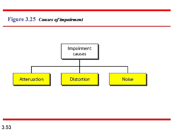
3 -4 TRANSMISSION IMPAIRMENT Signals travel through transmission media, which are not perfect. The imperfection causes signal impairment. This means that the signal at the beginning of the medium is not the same as the signal at the end of the medium. What is sent is not what is received. Three causes of impairment are attenuation, distortion, and noise. Topics discussed in this section: Attenuation Distortion Noise 3. 52

Figure 3. 25 Causes of impairment 3. 53

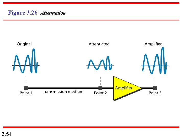
Figure 3. 26 Attenuation 3. 54

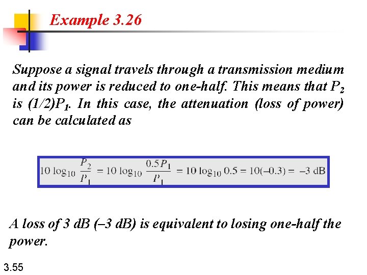
Example 3. 26 Suppose a signal travels through a transmission medium and its power is reduced to one-half. This means that P 2 is (1/2)P 1. In this case, the attenuation (loss of power) can be calculated as A loss of 3 d. B (– 3 d. B) is equivalent to losing one-half the power. 3. 55

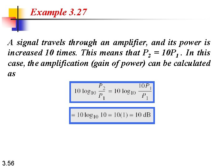
Example 3. 27 A signal travels through an amplifier, and its power is increased 10 times. This means that P 2 = 10 P 1. In this case, the amplification (gain of power) can be calculated as 3. 56

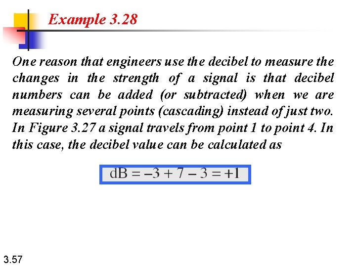
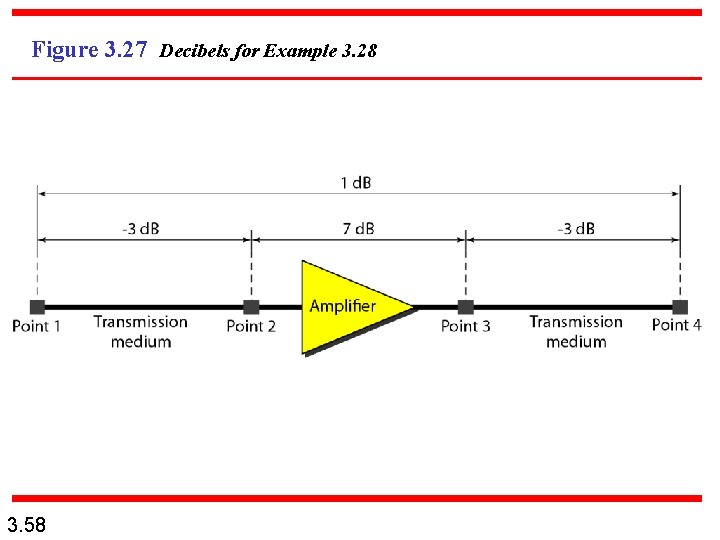
Example 3. 28 One reason that engineers use the decibel to measure the changes in the strength of a signal is that decibel numbers can be added (or subtracted) when we are measuring several points (cascading) instead of just two. In Figure 3. 27 a signal travels from point 1 to point 4. In this case, the decibel value can be calculated as 3. 57

Figure 3. 27 Decibels for Example 3. 28 3. 58

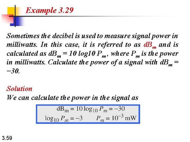
Example 3. 29 Sometimes the decibel is used to measure signal power in milliwatts. In this case, it is referred to as d. Bm and is calculated as d. Bm = 10 log 10 Pm , where Pm is the power in milliwatts. Calculate the power of a signal with d. Bm = − 30. Solution We can calculate the power in the signal as 3. 59

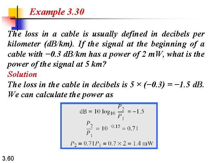
Example 3. 30 The loss in a cable is usually defined in decibels per kilometer (d. B/km). If the signal at the beginning of a cable with − 0. 3 d. B/km has a power of 2 m. W, what is the power of the signal at 5 km? Solution The loss in the cable in decibels is 5 × (− 0. 3) = − 1. 5 d. B. We can calculate the power as 3. 60

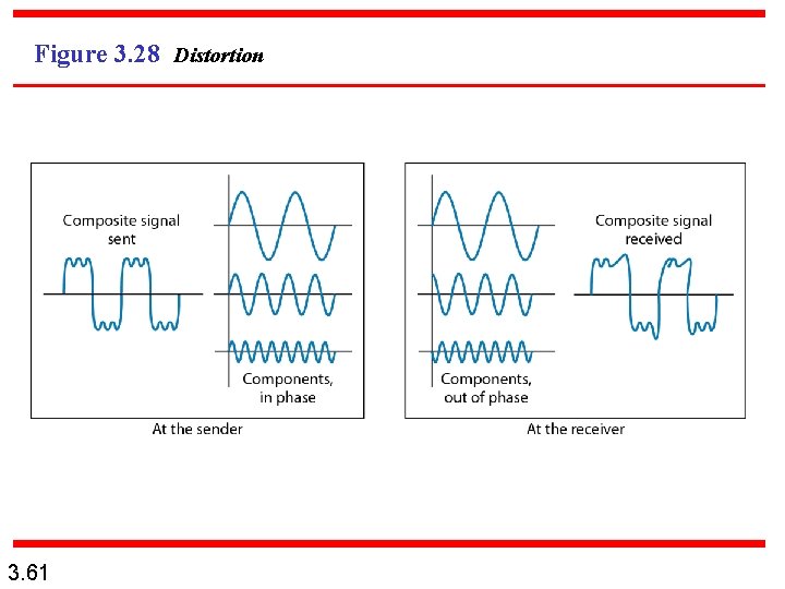
Figure 3. 28 Distortion 3. 61

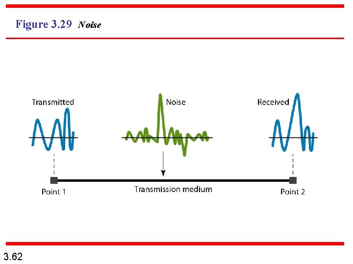
Figure 3. 29 Noise 3. 62

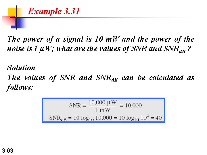
Example 3. 31 The power of a signal is 10 m. W and the power of the noise is 1 μW; what are the values of SNR and SNRd. B ? Solution The values of SNR and SNRd. B can be calculated as follows: 3. 63

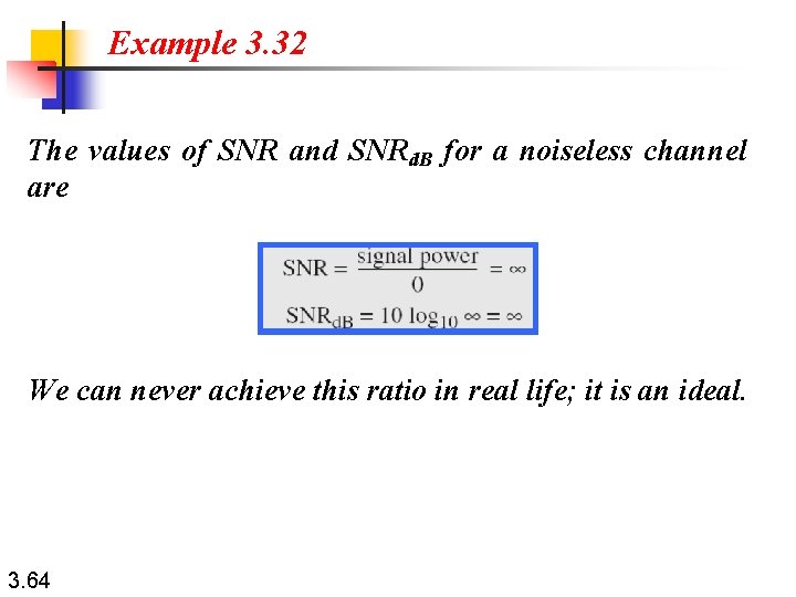
Example 3. 32 The values of SNR and SNRd. B for a noiseless channel are We can never achieve this ratio in real life; it is an ideal. 3. 64

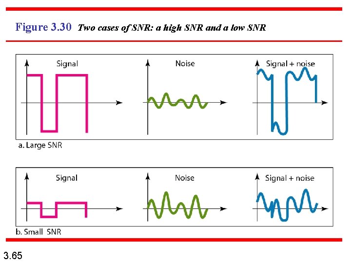
Figure 3. 30 Two cases of SNR: a high SNR and a low SNR 3. 65

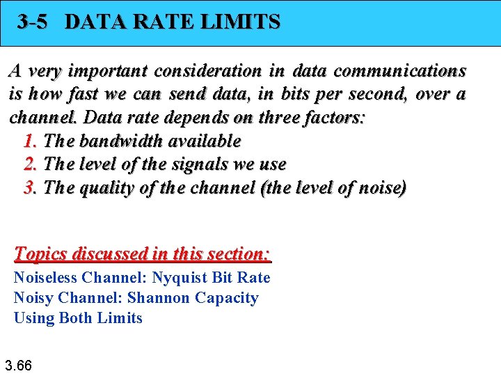
3 -5 DATA RATE LIMITS A very important consideration in data communications is how fast we can send data, in bits per second, over a channel. Data rate depends on three factors: 1. The bandwidth available 2. The level of the signals we use 3. The quality of the channel (the level of noise) Topics discussed in this section: Noiseless Channel: Nyquist Bit Rate Noisy Channel: Shannon Capacity Using Both Limits 3. 66

Note Increasing the levels of a signal may reduce the reliability of the system. 3. 67

Example 3. 33 Does the Nyquist theorem bit rate agree with the intuitive bit rate described in baseband transmission? Solution They match when we have only two levels. We said, in baseband transmission, the bit rate is 2 times the bandwidth if we use only the first harmonic in the worst case. However, the Nyquist formula is more general than what we derived intuitively; it can be applied to baseband transmission and modulation. Also, it can be applied when we have two or more levels of signals. 3. 68

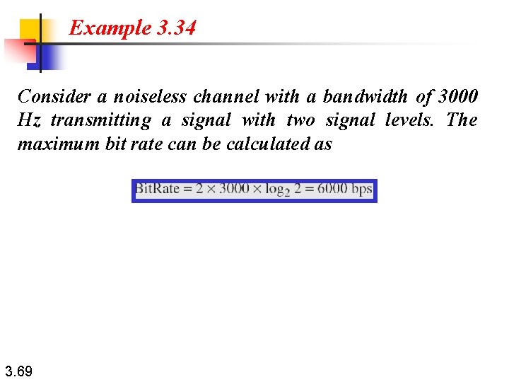
Example 3. 34 Consider a noiseless channel with a bandwidth of 3000 Hz transmitting a signal with two signal levels. The maximum bit rate can be calculated as 3. 69

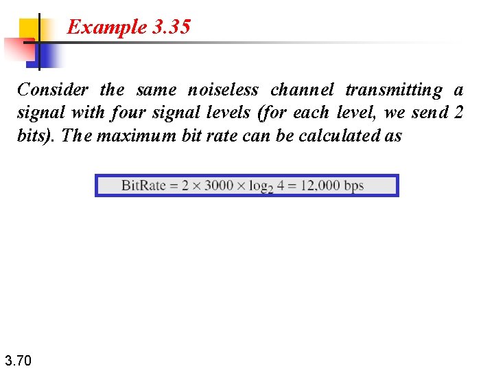
Example 3. 35 Consider the same noiseless channel transmitting a signal with four signal levels (for each level, we send 2 bits). The maximum bit rate can be calculated as 3. 70

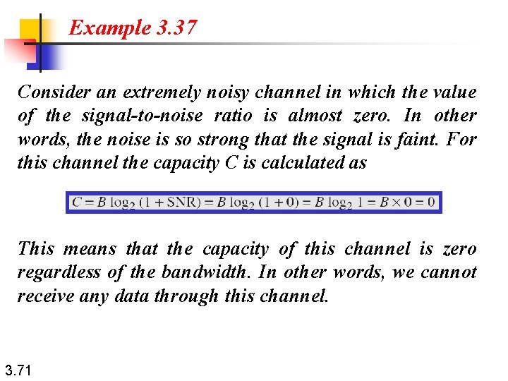
Example 3. 37 Consider an extremely noisy channel in which the value of the signal-to-noise ratio is almost zero. In other words, the noise is so strong that the signal is faint. For this channel the capacity C is calculated as This means that the capacity of this channel is zero regardless of the bandwidth. In other words, we cannot receive any data through this channel. 3. 71

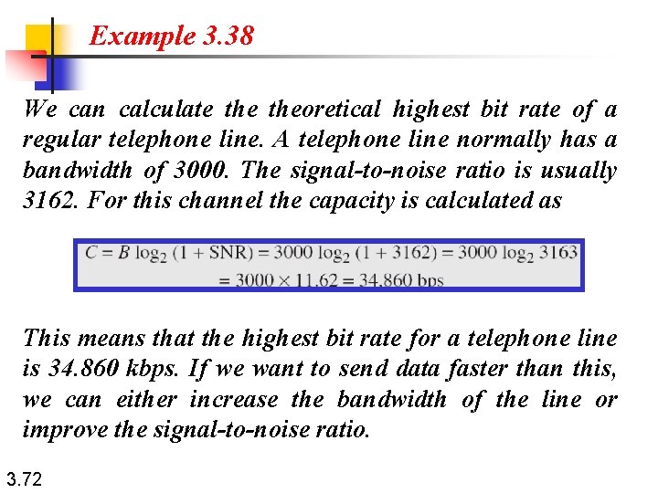
Example 3. 38 We can calculate theoretical highest bit rate of a regular telephone line. A telephone line normally has a bandwidth of 3000. The signal-to-noise ratio is usually 3162. For this channel the capacity is calculated as This means that the highest bit rate for a telephone line is 34. 860 kbps. If we want to send data faster than this, we can either increase the bandwidth of the line or improve the signal-to-noise ratio. 3. 72

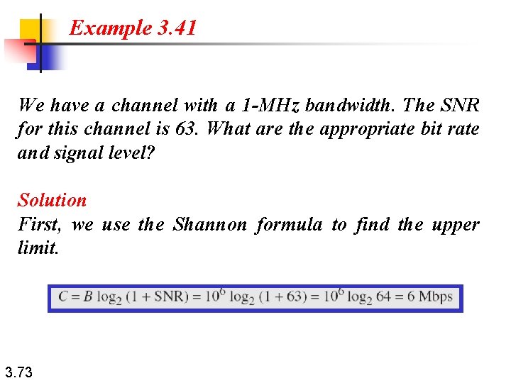
Example 3. 41 We have a channel with a 1 -MHz bandwidth. The SNR for this channel is 63. What are the appropriate bit rate and signal level? Solution First, we use the Shannon formula to find the upper limit. 3. 73

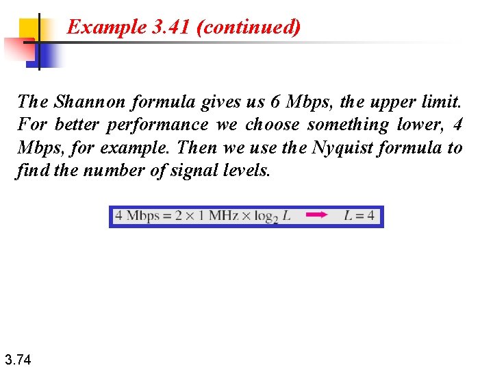
Example 3. 41 (continued) The Shannon formula gives us 6 Mbps, the upper limit. For better performance we choose something lower, 4 Mbps, for example. Then we use the Nyquist formula to find the number of signal levels. 3. 74

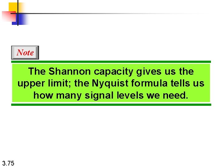
Note The Shannon capacity gives us the upper limit; the Nyquist formula tells us how many signal levels we need. 3. 75