Chapter 11 Logic Languages Programming Language Pragmatics Michael

Chapter 11 : : Logic Languages Programming Language Pragmatics Michael L. Scott Copyright © 2009 Elsevier

Logic Programming • The “other” principle declarative paradigm • Based in logic, which most of us see primarily in architecture and digital circuits • Arose as a programming paradigm in the 1970’s – due largely to the work of Cordell Green, Bertram Raphael, and others • Based on the methods of proof and logical inference, so appealing from the correctness standpoint – Real origins are in predicate calculus, in the same way that functional programming is based on lambda Copyright © 2009 Elsevier calculus

Logic Programming • Based on predicate calculus • Predicates - building-blocks P(x 1, x 2, . . . , x. K) – limit(f, infinity, 0) – enrolled(you, CS 344) • These are simply true/false statements that are based on their inputs. Copyright © 2009 Elsevier

Logic Programming Concepts • Operators: conjunction, disjunction, negation, implication – – P(x) and Q(x) P(y) or Q(z) Not P(x) implies Q(x) • You saw these (and more) in 135, and probably in other places where working on architecture or truth tables. Copyright © 2009 Elsevier

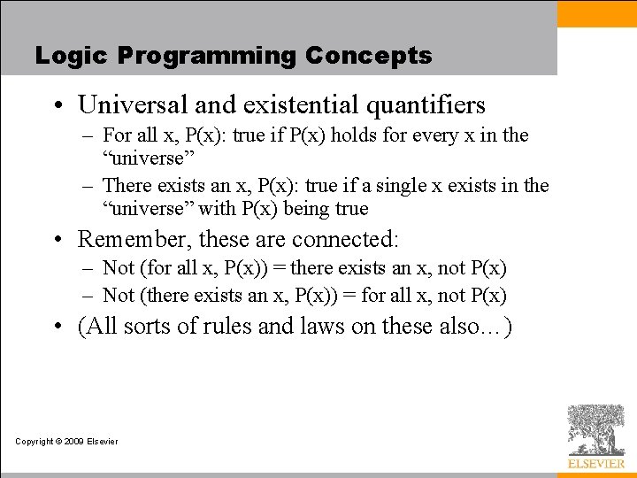
Logic Programming Concepts • Universal and existential quantifiers – For all x, P(x): true if P(x) holds for every x in the “universe” – There exists an x, P(x): true if a single x exists in the “universe” with P(x) being true • Remember, these are connected: – Not (for all x, P(x)) = there exists an x, not P(x) – Not (there exists an x, P(x)) = for all x, not P(x) • (All sorts of rules and laws on these also…) Copyright © 2009 Elsevier

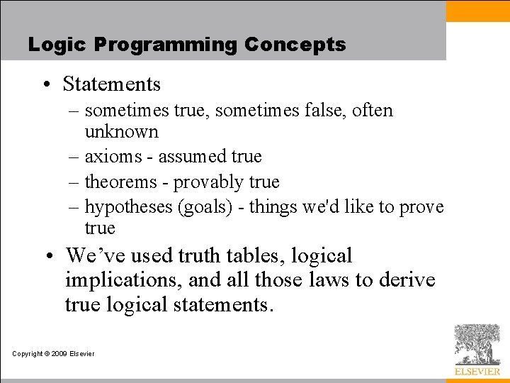
Logic Programming Concepts • Statements – sometimes true, sometimes false, often unknown – axioms - assumed true – theorems - provably true – hypotheses (goals) - things we'd like to prove true • We’ve used truth tables, logical implications, and all those laws to derive true logical statements. Copyright © 2009 Elsevier

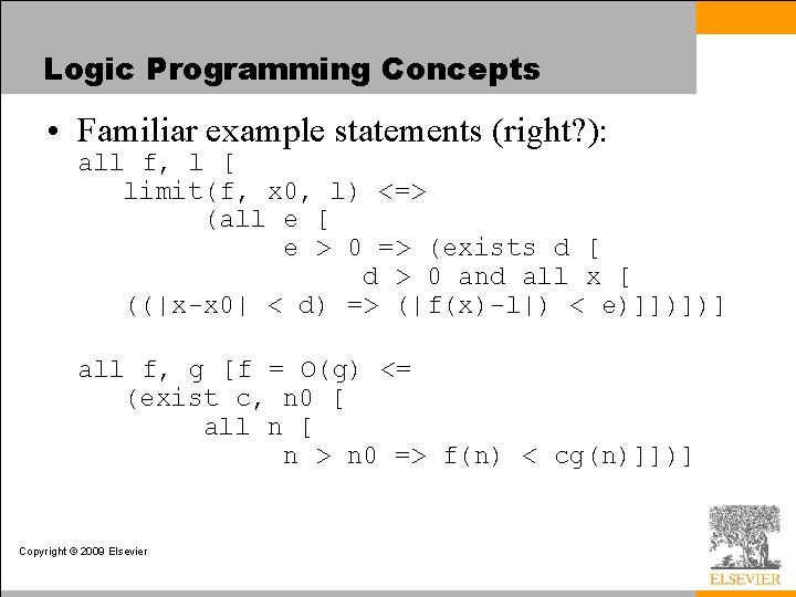
Logic Programming Concepts • Familiar example statements (right? ): all f, l [ limit(f, x 0, l) <=> (all e [ e > 0 => (exists d [ d > 0 and all x [ ((|x-x 0| < d) => (|f(x)-l|) < e)]])])] all f, g [f = O(g) <= (exist c, n 0 [ all n [ n > n 0 => f(n) < cg(n)]])] Copyright © 2009 Elsevier

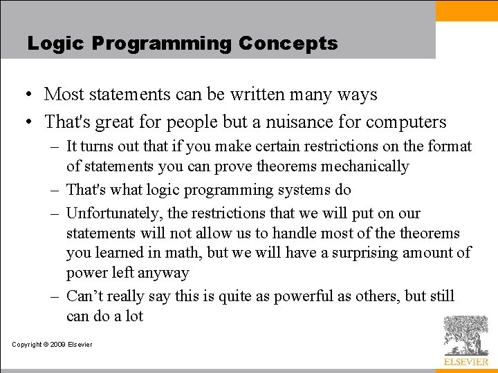
Logic Programming Concepts • Most statements can be written many ways • That's great for people but a nuisance for computers – It turns out that if you make certain restrictions on the format of statements you can prove theorems mechanically – That's what logic programming systems do – Unfortunately, the restrictions that we will put on our statements will not allow us to handle most of theorems you learned in math, but we will have a surprising amount of power left anyway – Can’t really say this is quite as powerful as others, but still can do a lot Copyright © 2009 Elsevier

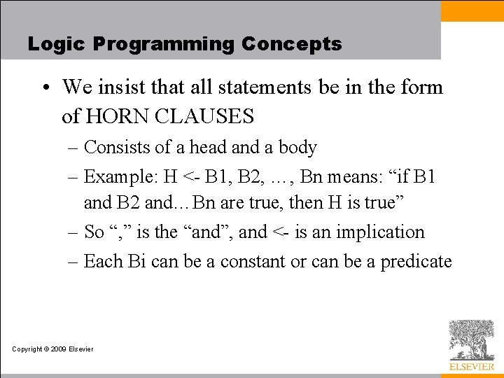
Logic Programming Concepts • We insist that all statements be in the form of HORN CLAUSES – Consists of a head and a body – Example: H <- B 1, B 2, …, Bn means: “if B 1 and B 2 and…Bn are true, then H is true” – So “, ” is the “and”, and <- is an implication – Each Bi can be a constant or can be a predicate Copyright © 2009 Elsevier

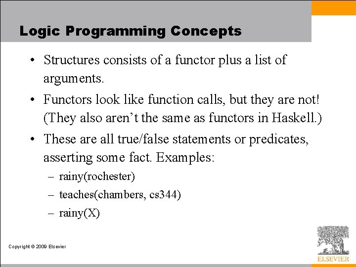
Logic Programming Concepts • Structures consists of a functor plus a list of arguments. • Functors look like function calls, but they are not! (They also aren’t the same as functors in Haskell. ) • These are all true/false statements or predicates, asserting some fact. Examples: – rainy(rochester) – teaches(chambers, cs 344) – rainy(X) Copyright © 2009 Elsevier

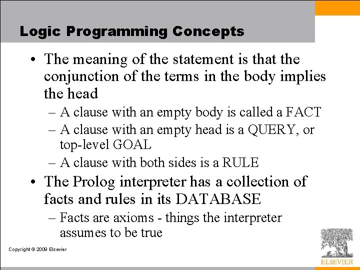
Logic Programming Concepts • The meaning of the statement is that the conjunction of the terms in the body implies the head – A clause with an empty body is called a FACT – A clause with an empty head is a QUERY, or top-level GOAL – A clause with both sides is a RULE • The Prolog interpreter has a collection of facts and rules in its DATABASE – Facts are axioms - things the interpreter assumes to be true Copyright © 2009 Elsevier

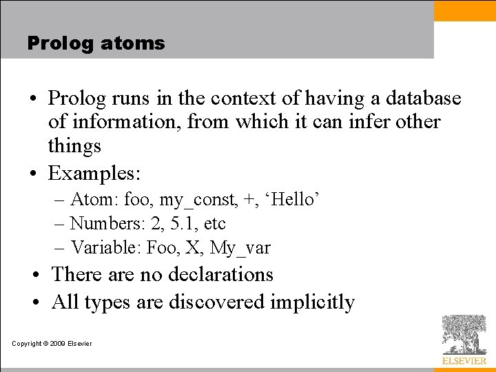
Prolog atoms • Prolog runs in the context of having a database of information, from which it can infer other things • Examples: – Atom: foo, my_const, +, ‘Hello’ – Numbers: 2, 5. 1, etc – Variable: Foo, X, My_var • There are no declarations • All types are discovered implicitly Copyright © 2009 Elsevier

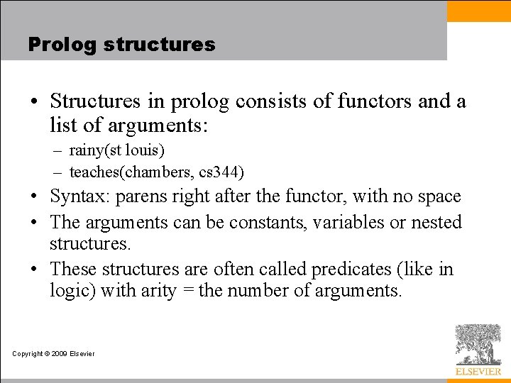
Prolog structures • Structures in prolog consists of functors and a list of arguments: – rainy(st louis) – teaches(chambers, cs 344) • Syntax: parens right after the functor, with no space • The arguments can be constants, variables or nested structures. • These structures are often called predicates (like in logic) with arity = the number of arguments. Copyright © 2009 Elsevier

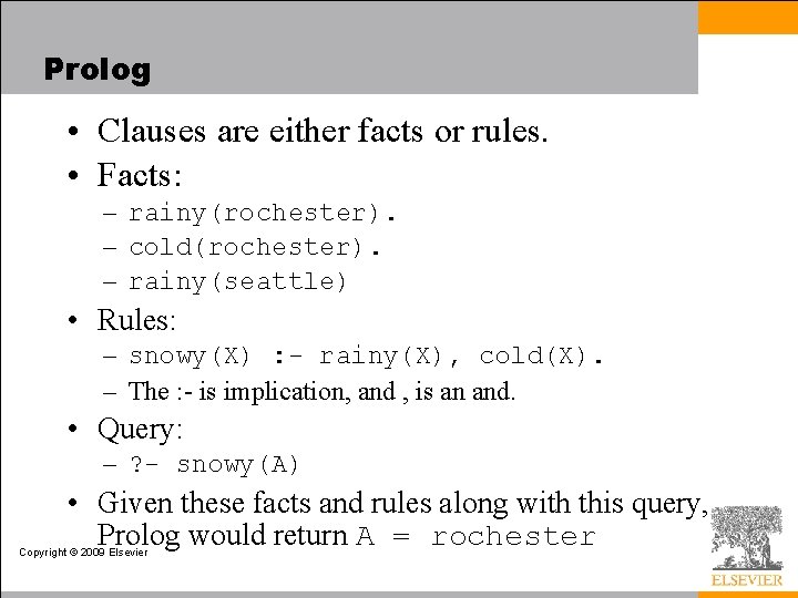
Prolog • Clauses are either facts or rules. • Facts: – rainy(rochester). – cold(rochester). – rainy(seattle) • Rules: – snowy(X) : - rainy(X), cold(X). – The : - is implication, and , is an and. • Query: – ? - snowy(A) • Given these facts and rules along with this query, Prolog would return A = rochester Copyright © 2009 Elsevier

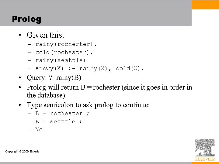
Prolog • Given this: – – rainy(rochester). cold(rochester). rainy(seattle) snowy(X) : - rainy(X), cold(X). • Query: ? - rainy(B) • Prolog will return B = rochester (since it goes in order in the database). • Type semicolon to ask prolog to continue: – B = rochester ; – B = seattle ; – No Copyright © 2009 Elsevier

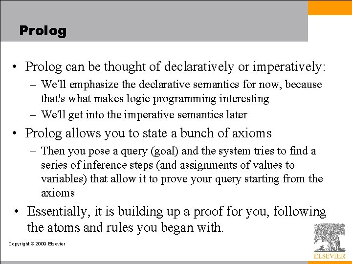
Prolog • Prolog can be thought of declaratively or imperatively: – We’ll emphasize the declarative semantics for now, because that's what makes logic programming interesting – We'll get into the imperative semantics later • Prolog allows you to state a bunch of axioms – Then you pose a query (goal) and the system tries to find a series of inference steps (and assignments of values to variables) that allow it to prove your query starting from the axioms • Essentially, it is building up a proof for you, following the atoms and rules you began with. Copyright © 2009 Elsevier

Prolog • Rules are theorems that allow the interpreter to infer things • To be interesting, rules generally contain variables employed(X) : - employs(Y, X). can be read: for all X, X is employed if there exists a Y such that Y employs X • Note the direction of the implication: – The example does NOT say that X is employed ONLY IF there is a Y that employs X Copyright © 2009 Elsevier

Prolog • The scope of a variable is the clause in which it appears – Variables whose first appearance is on the left hand side of the clause have implicit universal quantifiers – Variables whose first appearance is in the body of the clause have implicit existential quantifiers • Similarly: Copyright © 2009 Elsevier

Prolog grandmother(A, C) : - mother(A, B), mother(B, C). can be read: for all A, C [A is the grandmother of C if there exists a B such that A is the mother of B and B is the mother of C]. We probably want another rule that says grandmother(A, C) : - mother(A, B), father(B, C). Copyright © 2009 Elsevier

Prolog • To run a Prolog program, one asks the interpreter a question – This is done by stating a theorem - asserting a predicate - which the interpreter tries to prove • If it can, it says yes • If it can't, it says no • If your predicate contained variables, the interpreter prints the values it had to give them to make the predicate true. Copyright © 2009 Elsevier

Prolog • The interpreter works by what is called BACKWARD CHAINING – It begins with the thing it is trying to prove and works backwards looking for things that would imply it, until it gets to facts • It is also possible in theory to work forward from the facts trying to see if any of the things you can prove from them are what you were looking for - that can be very timeconsuming – Fancier logic languages use both kinds of chaining, with special smarts or hints from the user to bound the searches Copyright © 2009 Elsevier

Prolog • The predicate you ask for is the interpreter's original GOAL – In an attempt to SATISFY that goal, it looks for facts or rules with which the goal can be UNIFIED – Any variables that do not yet have values but which correspond to constants or to variables with values in the other clause get INSTANTIATED with that value – Anyplace where uninstantiated variables correspond, those variables are identified with each other, but remain without values Copyright © 2009 Elsevier

Prolog • The interpreter starts at the beginning of your database (this ordering is part of Prolog, NOT of logic programming in general) and looks for something with which to unify the current goal – If it finds a fact, great; it succeeds – If it finds a rule, it attempts to satisfy the terms in the body of the rule depth first – This process is motivated by the RESOLUTION PRINCIPLE, due to Robinson: • It says that if C 1 and C 2 are Horn clauses, where C 2 represents a true statement and the head of C 2 unifies with one of the terms in the body of C 1, then we can replace the term in C 1 with the body of C 2 to obtain another statement that is true if and only if C 1 is true Copyright © 2009 Elsevier

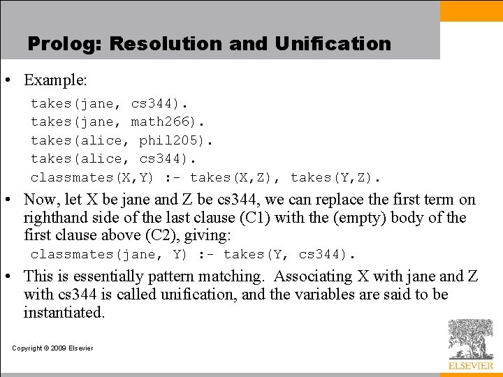
Prolog: Resolution and Unification • Example: takes(jane, cs 344). takes(jane, math 266). takes(alice, phil 205). takes(alice, cs 344). classmates(X, Y) : - takes(X, Z), takes(Y, Z). • Now, let X be jane and Z be cs 344, we can replace the first term on righthand side of the last clause (C 1) with the (empty) body of the first clause above (C 2), giving: classmates(jane, Y) : - takes(Y, cs 344). • This is essentially pattern matching. Associating X with jane and Z with cs 344 is called unification, and the variables are said to be instantiated. Copyright © 2009 Elsevier

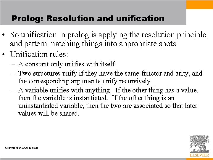
Prolog: Resolution and unification • So unification in prolog is applying the resolution principle, and pattern matching things into appropriate spots. • Unification rules: – A constant only unifies with itself – Two structures unify if they have the same functor and arity, and the corresponding arguments unify recursively – A variable unifies with anything. If the other thing has a value, then the variable is instantiated. If the other thing is an uninstantiated variable, then the two are associated so that later values will be shared. Copyright © 2009 Elsevier

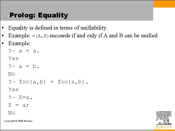
Prolog: Equality • Equality is defined in terms of unifiability. • Example: =(A, B)succeeds if and only if A and B can be unified • Example: ? - a = a. Yes ? - a = b. No ? - foo(a, b) = foo(a, b). Yes ? - X=a. X = a; No Copyright © 2009 Elsevier

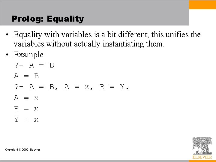
Prolog: Equality • Equality with variables is a bit different; this unifies the variables without actually instantiating them. • Example: ? - A = B, A = x, B = Y. A = x B = x Y = x Copyright © 2009 Elsevier

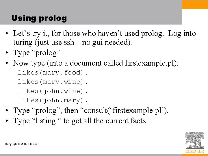
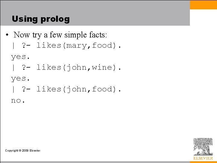
Using prolog • Let’s try it, for those who haven’t used prolog. Log into turing (just use ssh – no gui needed). • Type “prolog” • Now type (into a document called firstexample. pl): likes(mary, food). likes(mary, wine). likes(john, mary). • Type “prolog”, then “consult(‘firstexample. pl’). • Type “listing. ” to get all the current facts. Copyright © 2009 Elsevier

Using prolog • Now try a few simple facts: | ? - likes(mary, food). yes. | ? - likes(john, wine). yes. | ? - likes(john, food). no. Copyright © 2009 Elsevier

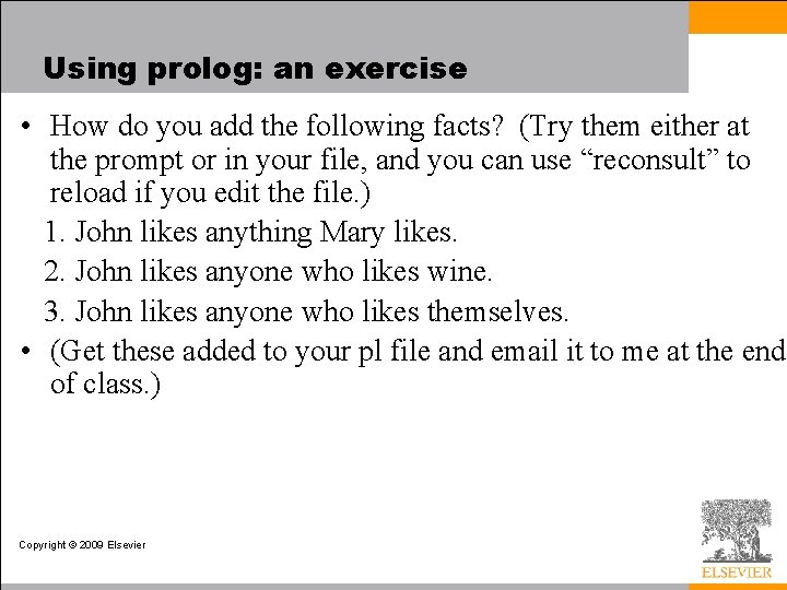
Using prolog: an exercise • How do you add the following facts? (Try them either at the prompt or in your file, and you can use “reconsult” to reload if you edit the file. ) 1. John likes anything Mary likes. 2. John likes anyone who likes wine. 3. John likes anyone who likes themselves. • (Get these added to your pl file and email it to me at the end of class. ) Copyright © 2009 Elsevier

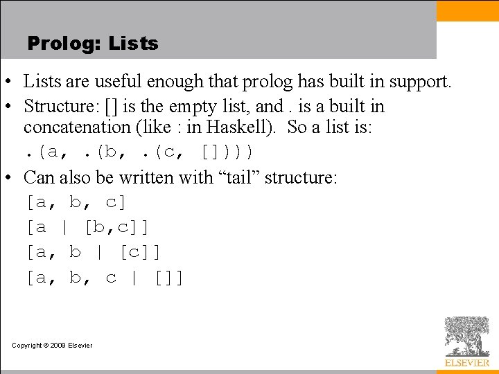
Prolog: Lists • Lists are useful enough that prolog has built in support. • Structure: [] is the empty list, and. is a built in concatenation (like : in Haskell). So a list is: . (a, . (b, . (c, []))) • Can also be written with “tail” structure: [a, b, c] [a | [b, c]] [a, b | [c]] [a, b, c | []] Copyright © 2009 Elsevier

Prolog: Lists • A demo: ? - [X|Y]=[[], dead(z), [2, [b, c]], [], Z]. X = [] Y = [dead(z), [2, [b, c]], [], Z] • Note: Z stayed unbound – some systems will represent this as _7800 in the last spot and then say Z = _7800. • Otherwise, variables bind as we expect. • Lists don’t have to be of same “type”, for any sense of type. Copyright © 2009 Elsevier

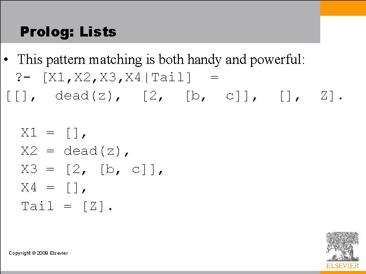
Prolog: Lists • This pattern matching is both handy and powerful: ? - [X 1, X 2, X 3, X 4|Tail] = [[], dead(z), [2, [b, c]], [], Z]. X 1 = X 2 = X 3 = X 4 = Tail [], dead(z), [2, [b, c]], [], = [Z]. Copyright © 2009 Elsevier

Prolog: Lists • List predicates: member(X, [X | _]). member(X, [_ | T]) : - member(x, T). sorted([]). sorted([_]). sorted([A, B | T]) : - A =< B, sorted([B | T]). Copyright © 2009 Elsevier

Prolog: Lists • Even crazier: append([], A, A). append([H | T], A, [H | L]) : append(T, A, L). • Now using it (note – prolog already has it coded!): ? - append([a, b, c], [d, e], L). L = [a, b, c, d, e] ? - append(X, [d, e], [a, b, c, d, e]). X = [a, b, c] ? - append([a, b, c], Y, [a, b, c, d, e]). Y = [d, e] Copyright © 2009 Elsevier

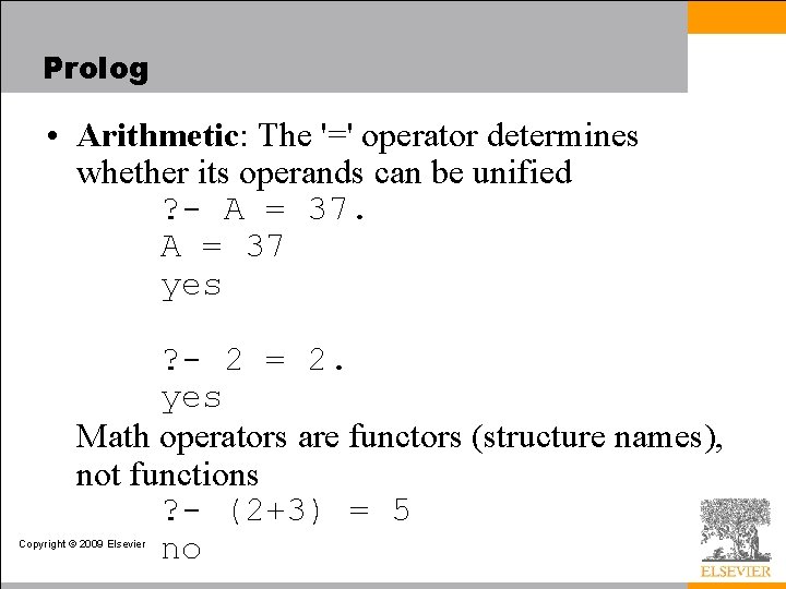
Prolog • Arithmetic: The '=' operator determines whether its operands can be unified ? - A = 37 yes ? - 2 = 2. yes Math operators are functors (structure names), not functions ? - (2+3) = 5 no Copyright © 2009 Elsevier

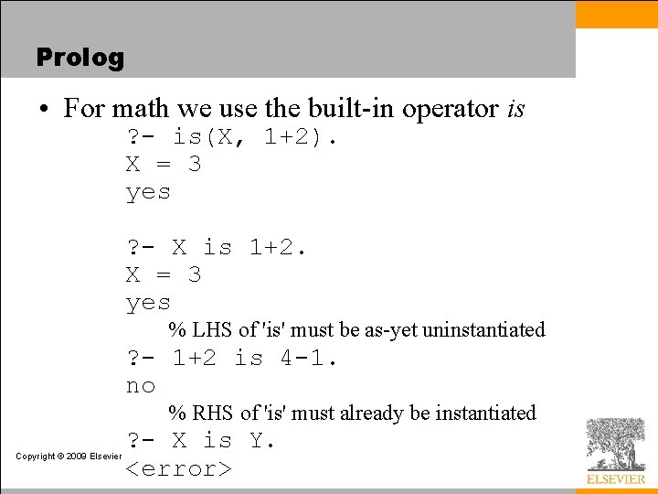
Prolog • For math we use the built-in operator is ? - is(X, 1+2). X = 3 yes ? - X is 1+2. X = 3 yes % LHS of 'is' must be as-yet uninstantiated ? - 1+2 is 4 -1. no % RHS of 'is' must already be instantiated Copyright © 2009 Elsevier ? - X is Y. <error>

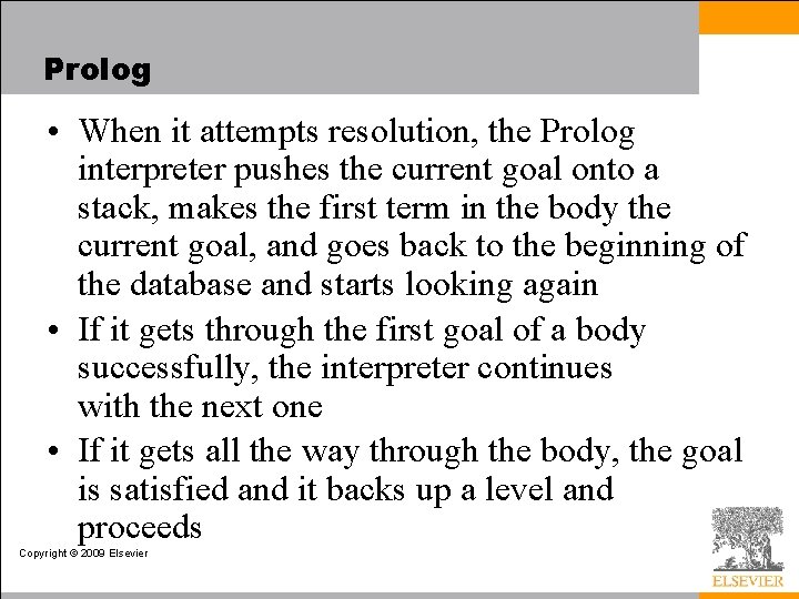
Prolog • When it attempts resolution, the Prolog interpreter pushes the current goal onto a stack, makes the first term in the body the current goal, and goes back to the beginning of the database and starts looking again • If it gets through the first goal of a body successfully, the interpreter continues with the next one • If it gets all the way through the body, the goal is satisfied and it backs up a level and proceeds Copyright © 2009 Elsevier

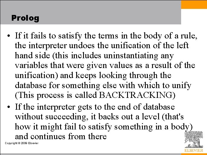
Prolog • If it fails to satisfy the terms in the body of a rule, the interpreter undoes the unification of the left hand side (this includes uninstantiating any variables that were given values as a result of the unification) and keeps looking through the database for something else with which to unify (This process is called BACKTRACKING) • If the interpreter gets to the end of database without succeeding, it backs out a level (that's how it might fail to satisfy something in a body) and continues from there Copyright © 2009 Elsevier

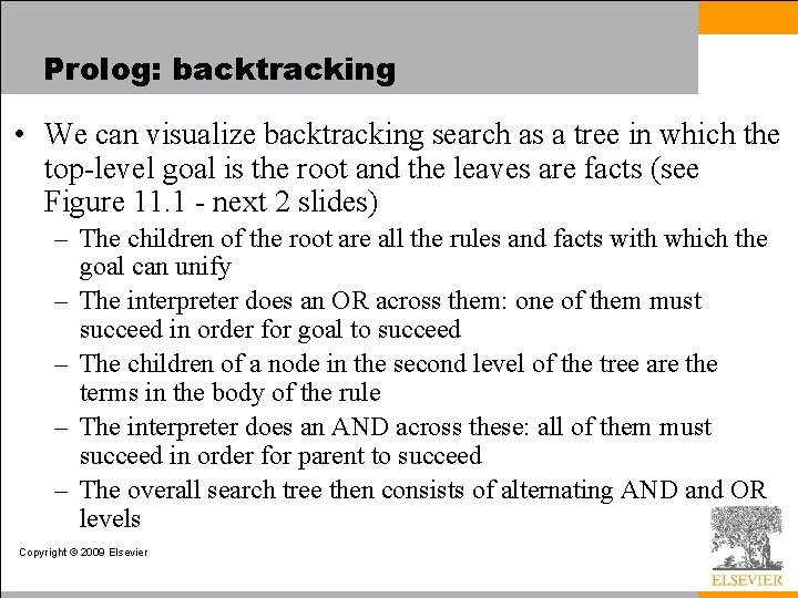
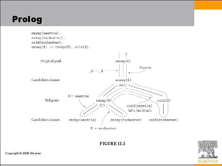
Prolog: backtracking • We can visualize backtracking search as a tree in which the top-level goal is the root and the leaves are facts (see Figure 11. 1 - next 2 slides) – The children of the root are all the rules and facts with which the goal can unify – The interpreter does an OR across them: one of them must succeed in order for goal to succeed – The children of a node in the second level of the tree are the terms in the body of the rule – The interpreter does an AND across these: all of them must succeed in order for parent to succeed – The overall search tree then consists of alternating AND and OR levels Copyright © 2009 Elsevier

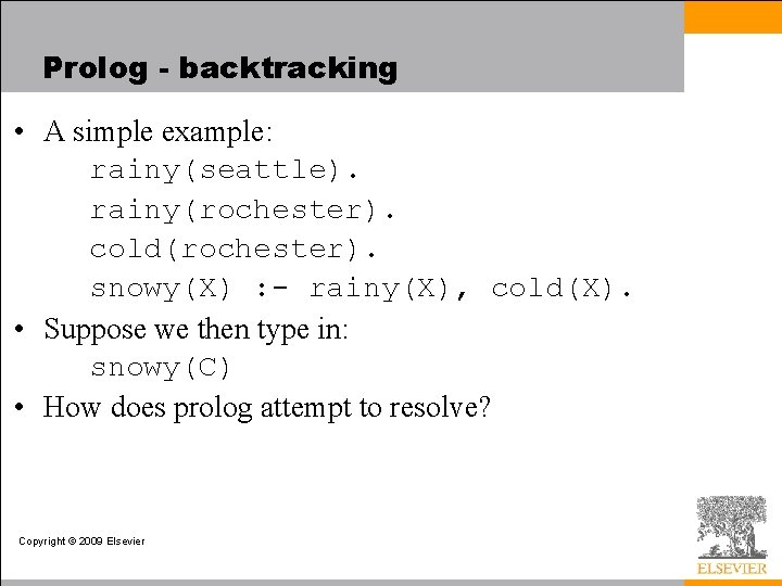
Prolog - backtracking • A simple example: rainy(seattle). rainy(rochester). cold(rochester). snowy(X) : - rainy(X), cold(X). • Suppose we then type in: snowy(C) • How does prolog attempt to resolve? Copyright © 2009 Elsevier

Prolog FIGURE 11. 1 Copyright © 2009 Elsevier

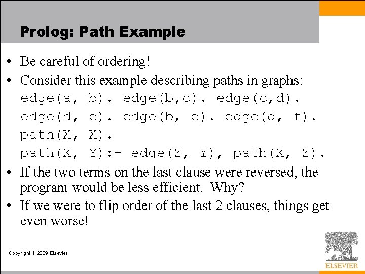
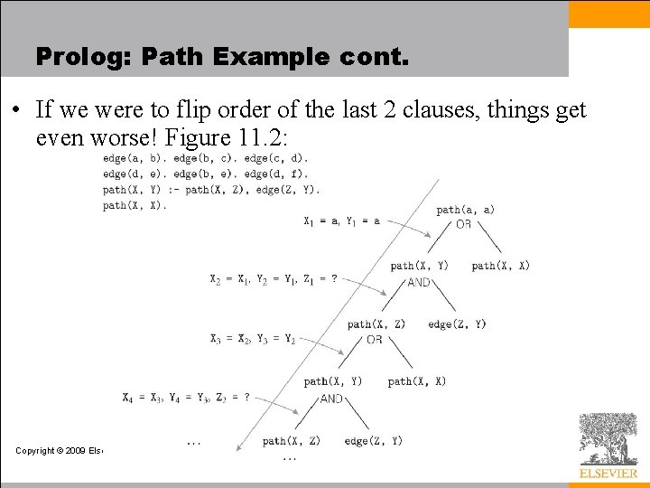
Prolog: Path Example • Be careful of ordering! • Consider this example describing paths in graphs: edge(a, b). edge(b, c). edge(c, d). edge(d, e). edge(b, e). edge(d, f). path(X, X). path(X, Y): - edge(Z, Y), path(X, Z). • If the two terms on the last clause were reversed, the program would be less efficient. Why? • If we were to flip order of the last 2 clauses, things get even worse! Copyright © 2009 Elsevier

Prolog: Path Example cont. • If we were to flip order of the last 2 clauses, things get even worse! Figure 11. 2: Copyright © 2009 Elsevier

Prolog • PROLOG IS NOT PURELY DECLARATIVE – The ordering of the database and the left-toright pursuit of sub-goals gives a deterministic imperative semantics to searching and backtracking – Changing the order of statements in the database can give you different results • It can lead to infinite loops • It can certainly result in inefficiency Copyright © 2009 Elsevier

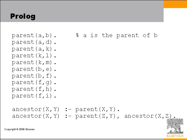
Prolog parent(a, b). parent(a, d). parent(a, k). parent(k, l). parent(k, m). parent(b, e). parent(b, f). parent(f, g). parent(f, h). parent(f, i). % a is the parent of b ancestor(X, Y) : - parent(X, Y). ancestor(X, Y) : - parent(Z, Y), ancestor(X, Z). Copyright © 2009 Elsevier

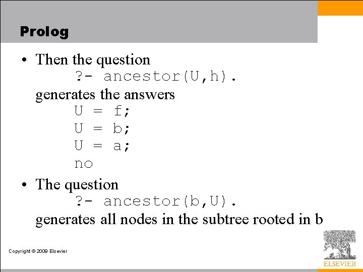
Prolog • Then the question ? - ancestor(U, h). generates the answers U = f; U = b; U = a; no • The question ? - ancestor(b, U). generates all nodes in the subtree rooted in b Copyright © 2009 Elsevier

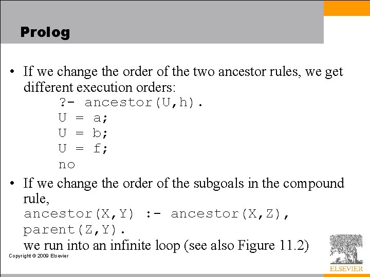
Prolog • If we change the order of the two ancestor rules, we get different execution orders: ? - ancestor(U, h). U = a; U = b; U = f; no • If we change the order of the subgoals in the compound rule, ancestor(X, Y) : - ancestor(X, Z), parent(Z, Y). we run into an infinite loop (see also Figure 11. 2) Copyright © 2009 Elsevier

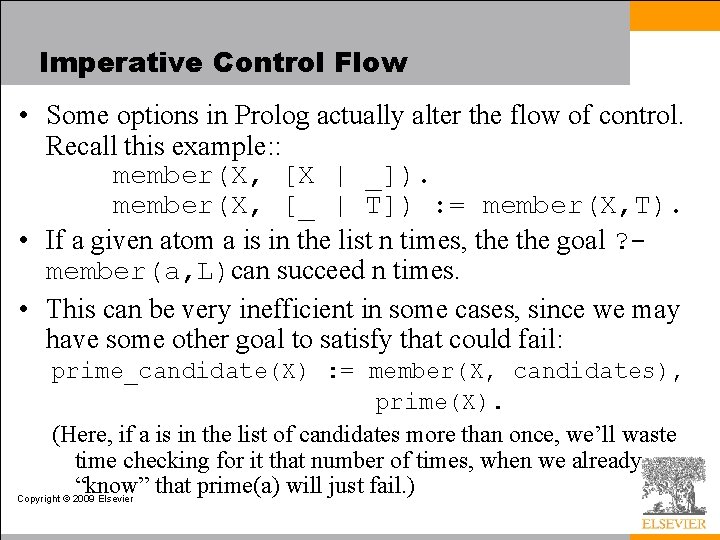
Imperative Control Flow • Some options in Prolog actually alter the flow of control. Recall this example: : member(X, [X | _]). member(X, [_ | T]) : = member(X, T). • If a given atom a is in the list n times, the goal ? member(a, L)can succeed n times. • This can be very inefficient in some cases, since we may have some other goal to satisfy that could fail: prime_candidate(X) : = member(X, candidates), prime(X). (Here, if a is in the list of candidates more than once, we’ll waste time checking for it that number of times, when we already “know” that prime(a) will just fail. ) Copyright © 2009 Elsevier

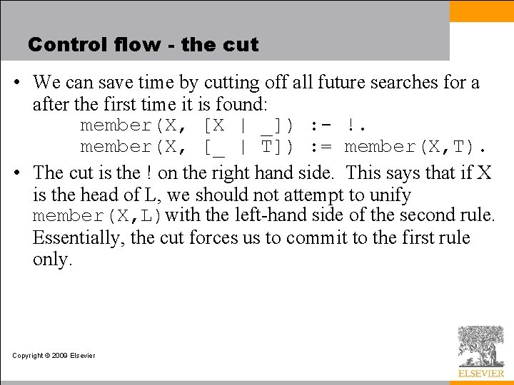
Control flow - the cut • We can save time by cutting off all future searches for a after the first time it is found: member(X, [X | _]) : - !. member(X, [_ | T]) : = member(X, T). • The cut is the ! on the right hand side. This says that if X is the head of L, we should not attempt to unify member(X, L)with the left-hand side of the second rule. Essentially, the cut forces us to commit to the first rule only. Copyright © 2009 Elsevier

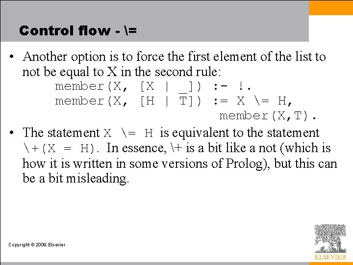
Control flow - = • Another option is to force the first element of the list to not be equal to X in the second rule: member(X, [X | _]) : - !. member(X, [H | T]) : = X = H, member(X, T). • The statement X = H is equivalent to the statement +(X = H). In essence, + is a bit like a not (which is how it is written in some versions of Prolog), but this can be a bit misleading. Copyright © 2009 Elsevier

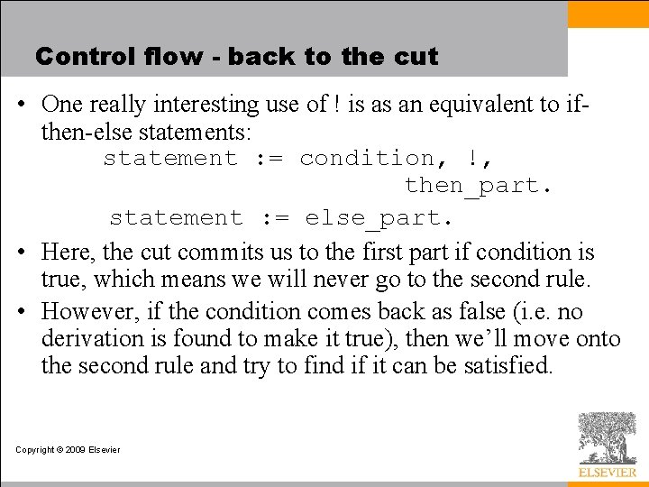
Control flow - back to the cut • One really interesting use of ! is as an equivalent to ifthen-else statements: statement : = condition, !, then_part. statement : = else_part. • Here, the cut commits us to the first part if condition is true, which means we will never go to the second rule. • However, if the condition comes back as false (i. e. no derivation is found to make it true), then we’ll move onto the second rule and try to find if it can be satisfied. Copyright © 2009 Elsevier

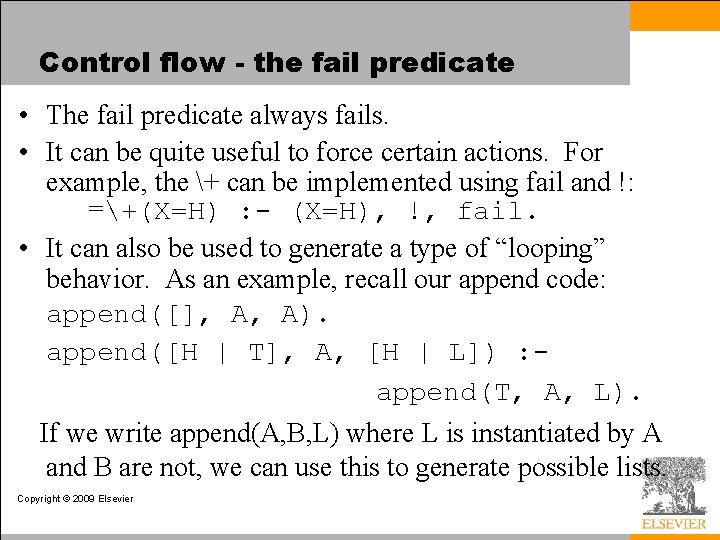
Control flow - the fail predicate • The fail predicate always fails. • It can be quite useful to force certain actions. For example, the + can be implemented using fail and !: =+(X=H) : - (X=H), !, fail. • It can also be used to generate a type of “looping” behavior. As an example, recall our append code: append([], A, A). append([H | T], A, [H | L]) : append(T, A, L). If we write append(A, B, L) where L is instantiated by A and B are not, we can use this to generate possible lists. Copyright © 2009 Elsevier

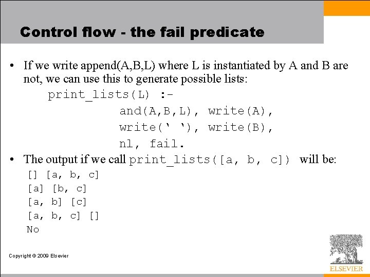
Control flow - the fail predicate • If we write append(A, B, L) where L is instantiated by A and B are not, we can use this to generate possible lists: print_lists(L) : and(A, B, L), write(A), write(‘ ‘), write(B), nl, fail. • The output if we call print_lists([a, b, c]) will be: [] [a, b, c] [a] [b, c] [a, b] [c] [a, b, c] [] No Copyright © 2009 Elsevier

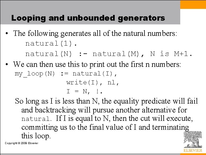
Looping and unbounded generators • The following generates all of the natural numbers: natural(1). natural(N) : - natural(M), N is M+1. • We can then use this to print out the first n numbers: my_loop(N) : = natural(I), write(I), nl, I = N, !. So long as I is less than N, the equality predicate will fail and backtracking will pursue another alternative for natural. If I is equal to N, then the cut will execute, committing us to the final value of I and terminating this loop. Copyright © 2009 Elsevier

Looping and unbounded generators • This programming idiom - an unbounded generator with a test-cut terminator - is know as generate-and-test. • This combination is generally used with side effects, such as I/O or modification of the database. • For example, we could use such a construct to add values to the database until some threshold is met. Copyright © 2009 Elsevier

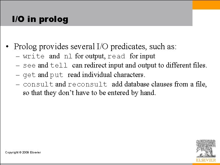
I/O in prolog • Prolog provides several I/O predicates, such as: – – write and nl for output, read for input see and tell can redirect input and output to different files. get and put read individual characters. consult and reconsult add database clauses from a file, so that they don’t have to be entered by hand. Copyright © 2009 Elsevier

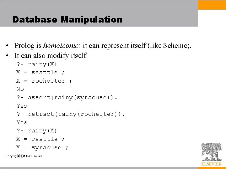
Database Manipulation • Prolog is homoiconic: it can represent itself (like Scheme). • It can also modify itself: ? - rainy(X) X = seattle ; X = rochester ; No ? - assert(rainy(syracuse)). Yes ? - retract(rainy(rochester)). Yes ? - rainy(X) X = seattle ; X = syracuse ; Copyright © 2009 Elsevier No

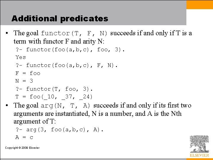
Additional predicates • The goal functor(T, F, N) succeeds if and only if T is a term with functor F and arity N: ? - functor(foo(a, b, c), foo, 3). Yes ? - functor(foo(a, b, c), F, N). F = foo N = 3 ? - functor(T, foo, 3). T = foo(_10, _37, _24) • The goal arg(N, T, A) succeeds if and only if its first two arguments are instantiated, N is a number, and A is the Nth argument of T: ? - arg(3, foo(a, b, c), A). A = c Copyright © 2009 Elsevier

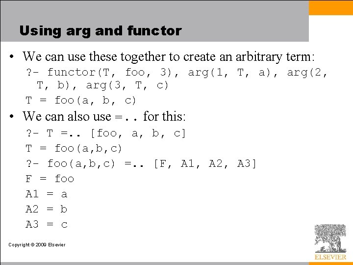
Using arg and functor • We can use these together to create an arbitrary term: ? - functor(T, foo, 3), arg(1, T, a), arg(2, T, b), arg(3, T, c) T = foo(a, b, c) • We can also use =. . for this: ? - T =. . [foo, a, b, c] T = foo(a, b, c) ? - foo(a, b, c) =. . [F, A 1, A 2, A 3] F = foo A 1 = a A 2 = b A 3 = c Copyright © 2009 Elsevier

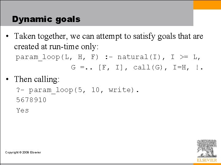
Dynamic goals • Taken together, we can attempt to satisfy goals that are created at run-time only: param_loop(L, H, F) : - natural(I), I >= L, G =. . [F, I], call(G), I=H, !. • Then calling: ? - param_loop(5, 10, write). 5678910 Yes Copyright © 2009 Elsevier

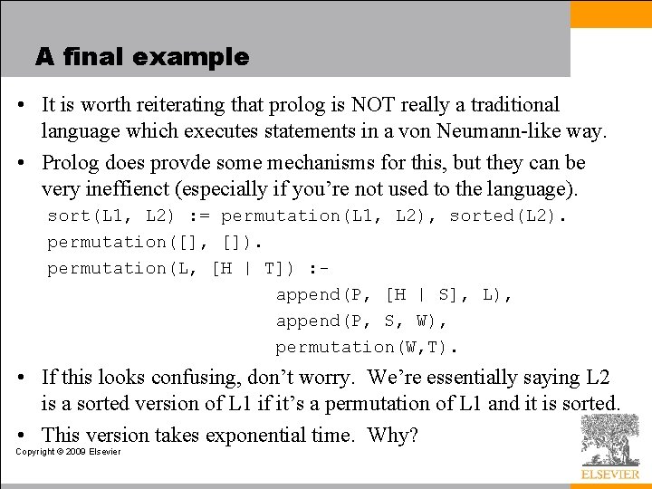
A final example • It is worth reiterating that prolog is NOT really a traditional language which executes statements in a von Neumann-like way. • Prolog does provde some mechanisms for this, but they can be very ineffienct (especially if you’re not used to the language). sort(L 1, L 2) : = permutation(L 1, L 2), sorted(L 2). permutation([], []). permutation(L, [H | T]) : append(P, [H | S], L), append(P, S, W), permutation(W, T). • If this looks confusing, don’t worry. We’re essentially saying L 2 is a sorted version of L 1 if it’s a permutation of L 1 and it is sorted. • This version takes exponential time. Why? Copyright © 2009 Elsevier

A final example: quicksort • Implementing something like quick sort is possible: quicksort([], []). quicksort([A, L 1], L 2) : - partition(A, L 1, P 1, S 1), quicksort(P 1, P 2), quicksort(S 1, S 2), append(P 2, [A | S 2], L 2). partition(A, [], []). partition(A, [H | T], [H | P], S) : - A >= H, partition(A, T, P, S). partition(A, [H | T], [P], [H | S]) : - A =< H, partition(A, T, P, S). Copyright © 2009 Elsevier

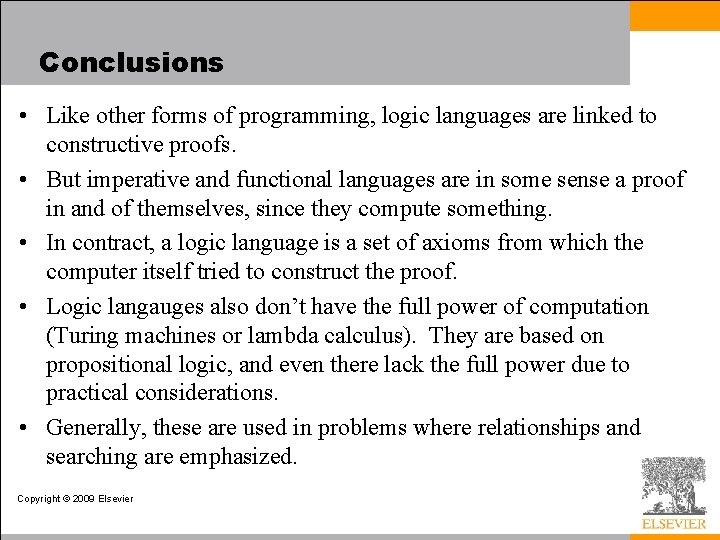
Conclusions • Like other forms of programming, logic languages are linked to constructive proofs. • But imperative and functional languages are in some sense a proof in and of themselves, since they compute something. • In contract, a logic language is a set of axioms from which the computer itself tried to construct the proof. • Logic langauges also don’t have the full power of computation (Turing machines or lambda calculus). They are based on propositional logic, and even there lack the full power due to practical considerations. • Generally, these are used in problems where relationships and searching are emphasized. Copyright © 2009 Elsevier

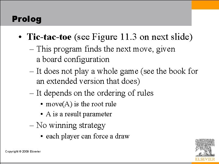
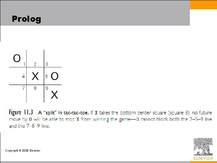
Prolog • Tic-tac-toe (see Figure 11. 3 on next slide) – This program finds the next move, given a board configuration – It does not play a whole game (see the book for an extended version that does) – It depends on the ordering of rules • move(A) is the root rule • A is a result parameter – No winning strategy • each player can force a draw Copyright © 2009 Elsevier

Prolog Copyright © 2009 Elsevier

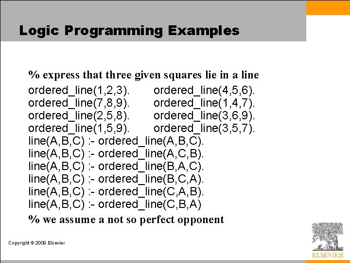
Logic Programming Examples % express that three given squares lie in a line ordered_line(1, 2, 3). ordered_line(4, 5, 6). ordered_line(7, 8, 9). ordered_line(1, 4, 7). ordered_line(2, 5, 8). ordered_line(3, 6, 9). ordered_line(1, 5, 9). ordered_line(3, 5, 7). line(A, B, C) : - ordered_line(A, C, B). line(A, B, C) : - ordered_line(B, A, C). line(A, B, C) : - ordered_line(B, C, A). line(A, B, C) : - ordered_line(C, A, B). line(A, B, C) : - ordered_line(C, B, A) % we assume a not so perfect opponent Copyright © 2009 Elsevier

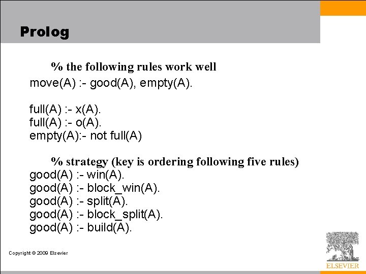
Prolog % the following rules work well move(A) : - good(A), empty(A). full(A) : - x(A). full(A) : - o(A). empty(A): - not full(A) % strategy (key is ordering following five rules) good(A) : - win(A). good(A) : - block_win(A). good(A) : - split(A). good(A) : - block_split(A). good(A) : - build(A). Copyright © 2009 Elsevier

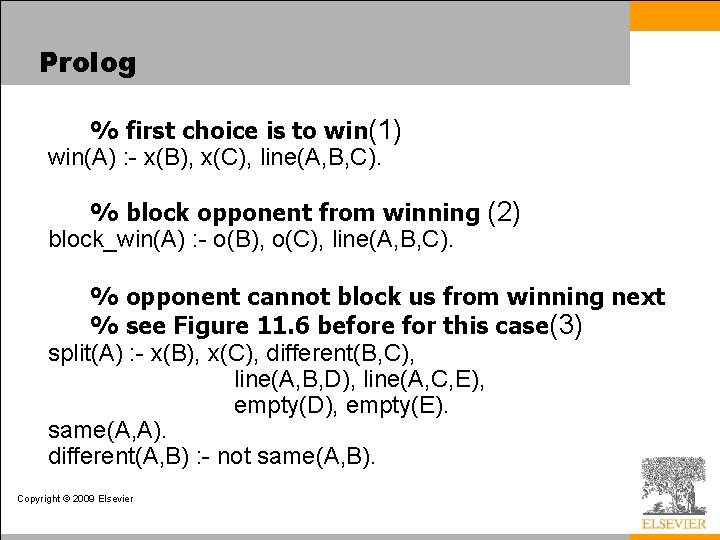
Prolog % first choice is to win(1) win(A) : - x(B), x(C), line(A, B, C). % block opponent from winning (2) block_win(A) : - o(B), o(C), line(A, B, C). % opponent cannot block us from winning next % see Figure 11. 6 before for this case(3) split(A) : - x(B), x(C), different(B, C), line(A, B, D), line(A, C, E), empty(D), empty(E). same(A, A). different(A, B) : - not same(A, B). Copyright © 2009 Elsevier

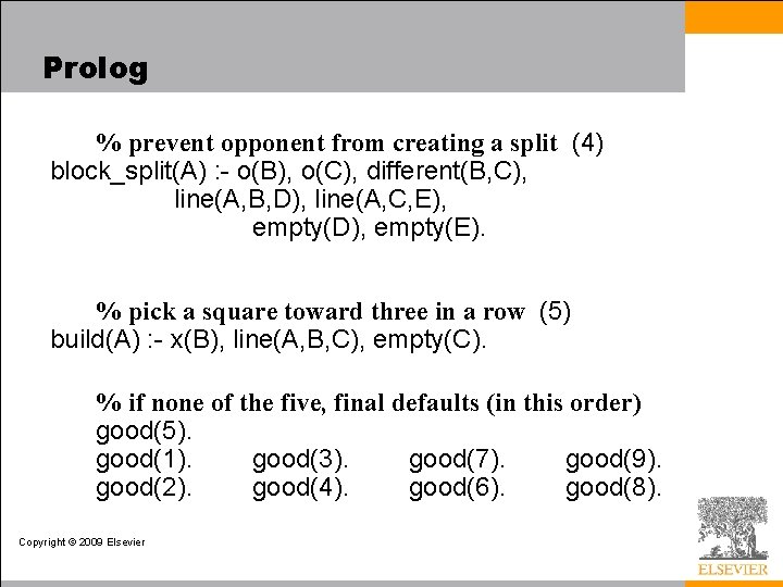
Prolog % prevent opponent from creating a split (4) block_split(A) : - o(B), o(C), different(B, C), line(A, B, D), line(A, C, E), empty(D), empty(E). % pick a square toward three in a row (5) build(A) : - x(B), line(A, B, C), empty(C). % if none of the five, final defaults (in this order) good(5). good(1). good(3). good(7). good(9). good(2). good(4). good(6). good(8). Copyright © 2009 Elsevier