Chap 9 Testing Hypotheses and Assessing Goodness of

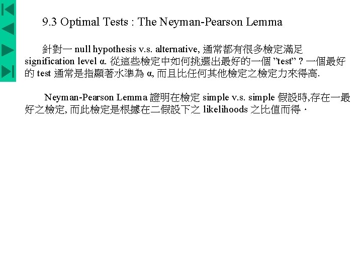
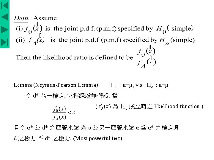
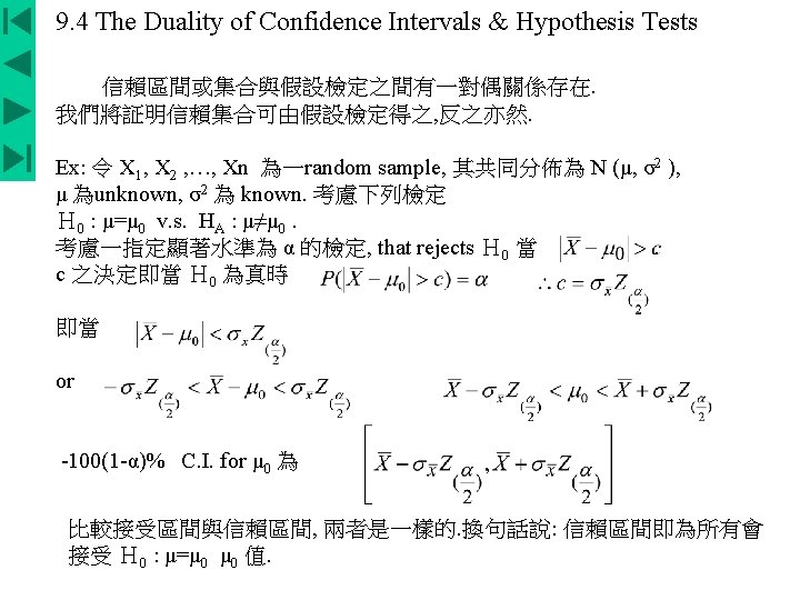
Chap 9 Testing Hypotheses and Assessing Goodness of Fit 統計假設檢定基本上是基於一分配所得之 random sample 來區分二分佈之 一種方法. 例: 給定 X 1, X 2 , …, Xn ~ i. i. d N (μ, σ2 ) 想決定 μ 究竟是 μ 1 或 μ 2 , 則為區分二分佈. 主要之架構: 理論根據 Neyman-Pearson Lemma 而來 H 0 : Null hypothesis (一般 H 0 取較為簡單或拒絕的結果為較嚴重的假設 ) H 1 : Alternative hypothesis Simple Hypotheses : 如H 0 : μ=μ 1 v. s. H 1 : μ=μ 2 Composite Hypothesis : H 0 : X 1, X 2 , …, Xn 來自Poisson(λ) H 1 : not Poisson(λ) 若 H 1 改為 P(λ 1) 則為 simple Hypothesis Ex: B (n, p) H 0 : p = 0. 50 v. s. H 1 : p = 0. 25 or H 1 : p ≠ 0. 5 ( two-sided alternative ) p ＜ 0. 5 ( one-sided alternative ) p ＞ 0. 5

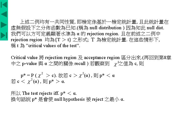
9. 2 The Neyman-Pearson Paradigm 根據 Neyman-Pearson 決定是否接受 null hyp. 是看檢定統計量 T(x) 是落在 acceptance region 或在 rejection region H 0 1. Type Ⅰ error : H 0 為真, 但 reject H 0. Accept P ( reject H 0 | H 0 is true ) = α Reject 若 H 0 為 simple, 稱 α 為 significance level. 若 H 0 為 composite, 則在每一特殊 θ 下有一 type Ⅰ error 此時 significance level 為 max P (Type Ⅰ error) 2. Type Ⅱ error : H 0 false, but accept H 0. P (accept H 0 | H 0 false) = β True False ˇ Type Ⅱ Type Ⅰ ˇ ‧Power function P (reject H 0 |θ) = 1 –β 與 θ 相關 理想狀況: α = β = 0 , 但除非是在 trivial case 下否則是不可能, 通常在樣本 數固定的情況下 α↓ 則 β↑. Neyman-Pearson 解決這種矛盾的方法是先將 significance level α 固定後, α 通常是很小的值, 再設法建造一 test 使 β 為最 小.

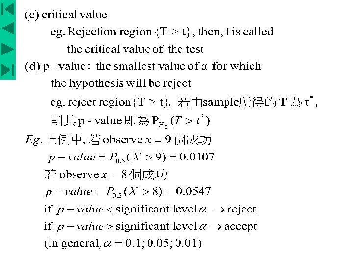
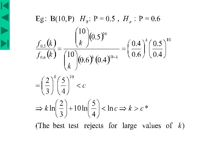
Ex. 設X ~ B (n, p) H 0 : p = 0. 5 v. s. HA : p ＞ 0. 5. 即 Rejection region 為由 X 中之大的值構成, 利用 binomial 之分佈表, 設 rejection region 為 {8, 9, 10}, 則 α = P (X ＞ 7 | p = 0. 5) = 1 – P (X ≦ 7) = 0. 0547 若 rejection region 為 {7, 8, 9, 10}, 則 α = P (X ≧ 7 | p = 0. 5) = 0. 172 The Neyman - Pearson approach 則先設定 α 之值. 如選 α= 0. 0547. 若 true value of p 為 0. 6. 1 - β(0. 6) = P(X ≧ 8 | p =0. 6) = 0. 1673 Power 隨著p增加 (即 遠離 H 0 : p = 0. 5) 而增加 1 - β(0. 7) = P(X ≧ 8 | p =0. 7) = 0. 3828

Ex. 再考慮前述檢定 goodness of fit to a Poisson dist. 虛無假設 : 數據來自於 Poisson dist. 對立假設 : 來自一未註明之 discrete dist. radioactive ======== α particles sources 放射性物質 在單位時間內所放射的 α 粒子數目為一隨機變數. 假設 (1) 在觀察時段中, (每個 atom 原子)其 emission rate 為一常數 (2) 所觀察的α particles數目, 來自於 a very large number of independent sources (atoms 原子) 對此 radioactive decay data, Poisson 模型為一 appropriate 的模型, Poisson postulate (i) the underlying rate at which the events occur is constant in space or in time (ii) events in disjoint intervals of space or time occur independently (iii) There are no multiple events.

Berkson (1966) 分析從美國國家標準局所獲得的 (1) 在連續的放射中紀錄10, 220次 Americium (2) observed mean emission rate 241 鋂 (Am, 原子序 95) = =0. 8396 (3) 準確度 (用於紀錄時間的 clock 可達 0. 0002秒) 表 Berkson 分析 1207 intervals, each of length 10秒. 見 : , 其中λ= 0. 8392 x 10 (秒) = 8. 932 (為Poisson的mean) P 1 = π0+π1+π2 P 16 = The joint distribution of the counts in all cells is multinomial with n = 1207 & probabilities P 1, P 2, …, P 16.

Goodness of Fit : Pearson’s chi-square statistic = (8. 99) d. f. = # of cells - # of indep. parameters o fitted -1 = 16 -1 -1 = 14 Fig. 8. 1 do not reject 亦可採用 generalized likelihood test, 即

k 0 1 2 3 4 7 8 9 10 9. 31 6. 21 4. 14 2. 76 1. 84 0. 55 0. 36 0. 24 0. 16

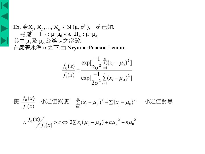
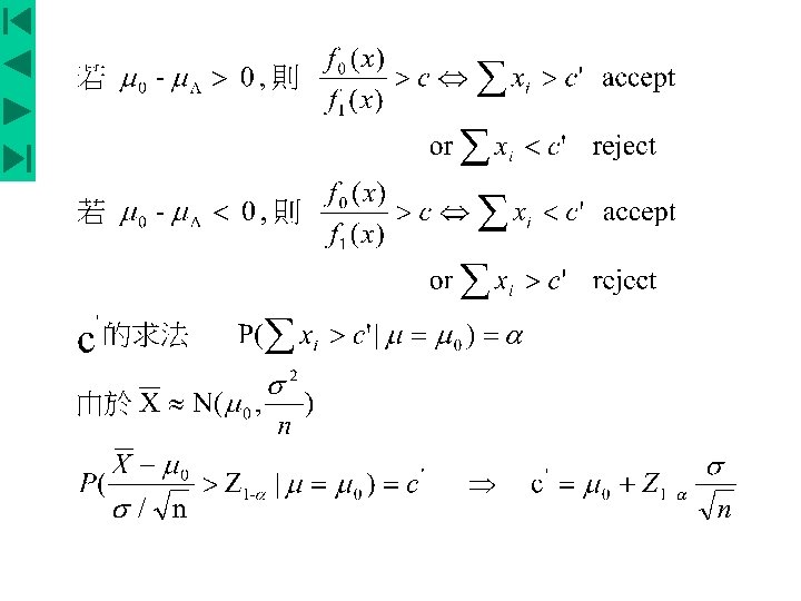
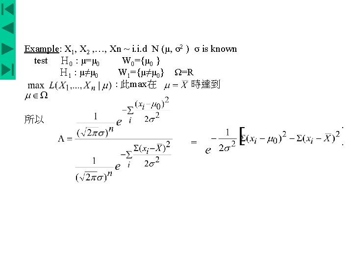
Eg. X 1, X 2 , …, Xn ~ i. i. d N (μ, σ2 ) σ is known Ｈ 0 : μ=μ 0 v. s. Ha : μ=μA Require signification level = α N-P Lemma Among all tests with signification level α, the test reject for is most powerful. 1. if μ 0 –μA ＞ 0, the likelihood ratio test is small if is small 2. if μ 0 –μA ＜ 0, the likelihood ratio test is small if is large Assumeμ 0 –μA ＜ 0, Now choose x 0 , s. t. power of this test

Def : if HA is composite, A test that is most powerful for every simple alternative in HA is said to be uniformly most powerful. Eg. : X 1, X 2 , …, Xn ~ i. i. d N (μ, σ2 ) Ｈ 0 : μ=μ 0 v. s. HA : μ＞μ 0 For a particular simple alternative μ=μA＞μ 0 , the most powerful test reject for with x 0 only depends on μ 0 , n &σ2 but not on μA. ∵ this test is most powerful & is the same for every simple alternative in HA , it is uniformly most powerful. 在檢定 Ｈ 0 : μ≦μ 0 v. s. HA : μ＞μ 0 時 上述檢定仍為uniformly most powerful 但在檢定 Ｈ 0 : μ=μ 0 v. s. HA : μ≠μ 0 時則非 UMP

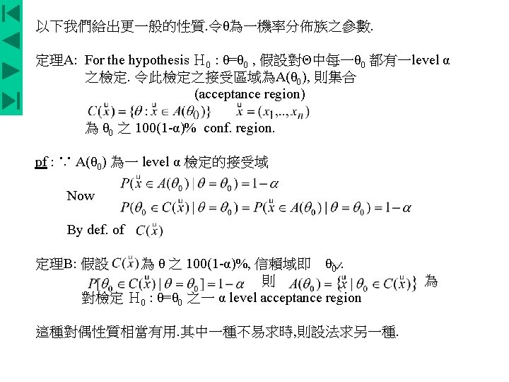
9. 5 Generalized Likelihood Ratio Tests (廣義概似比檢定) (i) 當 hypothesis is simple v. s. simple 時 likelihood ratio test is optimal. (ii) 當 hypotheses 不是 simple 時, 我們發展一 likelihood ratio test 之推廣 test. 稱為 generalized likelihood ratio test. 這種 tests 一般不見得為 optimal, 但 在沒有任何 tests 為 optimal 時, 它的表現一般而言, 是還不錯的. Generalized likelihood ratio tests 有很多好處, 它們所扮演的角色就像估計 中的 M. L. E. 一樣 令 X = (X 1, X 2 , …, Xn) 之 joint p. d. f. 為 L (X 1, X 2 , …, Xn |θ) 則 Ｈ 0 可能為 , W 0 為一所有可能之 θ 之一 subset , 考慮

Λ* 值小時, 即對 Ｈ 0 不利. 為了計算上之方便改用下列 test: 令 ∴ Λ = min (Λ*, 1) Λ*小時, Λ亦小 The rejection region for a likelihood ratio tests consists of small values of Λ, 如所有Λ≦λ 0

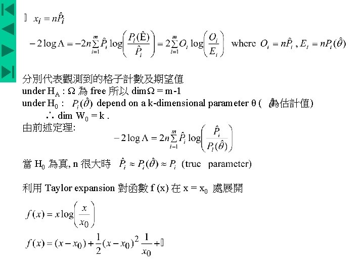
9. 6 Likelihood Ratio Tests for the Multinomial Distribution 在 multinomial goodness-of-fit test 中, 虛無假設 H 0 : P = P (θ) W 0 , 其中 P 為 cell prob. 向量, θ 為參數 HA : H 0 not true likelihood ratio 之分子部份. 其中 xi 為 m 格子中之觀測計數. 由 M. L. E. 之定義: 一 M. L. E. 即為使 Likelihood function 為最大之 θ. ∴相對應 之 Pi 值以 表之. 由於 P Ω 時, 沒有 以外之限制 所以 the likelihood ratio 為

= 0 second term on the right hand side. 此檢定即為前面 8. 2節中提到的 Pearson’s -test for goodness of fit. 而 Pearson’s -test for goodness of fit 通常較常被用. 因為計算上比較容易.

Ex : (Hardy-Weinberg Equilibrium) Genotype AA Aa aa (1 -θ)2 2θ(1 -θ) M. L. E. of θ Blood Type M θ 2 MN N Observed 342 500 187 Expected 340. 6 502. 8 185. 6 H 0 : as special above. H 1 : the multinomial dist. does not have the probability specified above. α= 0. 05 = 0. 00575 + 0. 01559 + 0. 01056 = 0. 0319

x 12 (0. 05) = 3. 84 do not reject H 0 x 2 (0. 76) = 0. 09 so the p-value 為 0. 76 p-value 之另一種解釋為在模型正確的假設下, 會出現此值之機率為 76%. The likelihood ratio test statistic 為 p-value 為 0. 86.

以下為 Bliss & Fisher (1953) 之表, 為在 400個方格上之計數. Number per square 0 1 2 3 4 5 6 7 8 9 10 19 Frequency 56 104 80 62 42 27 9 9 5 3 2 1 Fit P (λ)中 λ 之M. C. E. 下表顯示 observed 及 expected counts 及 chi-square test stat. 之計算值. 最後 幾 個格子則集合在一起, 使得 expected counts 不致太小, 靠近 5. Observed 56 10 4 80 62 42 27 9 20 Expected 34. 85. 10 84. 51. 25. 10. 5. 0 9 1 3. 8 4 5 1 2 Component 12. 4. 2 5. 5 6. 0 1. 8 0. 1 45. of X 2 8 4 4 0 x 2 = 75. 6 ∵x 62 (0. 005) = 18. 55 d. f. =6=8 -1 -1 p-value ＜ 0. 005 rejects H 0 model fails 之原因來自第一格及最後一格, 太多小的及太多大的.

Ex C. (Fisher’s Reexamination of Mendel’s Data) 在孟德爾許多有名的實驗中, 其中一個實驗是將 smooth, yellow (平滑, 黃色) 的 male peas, 與 wrinkled, green (皺, 綠色) 的 female peas 相配. 根據現在的基因 理論. 子孫的相對頻率應為: Type Frequency Observed count Expected count Smooth-yellow 3/4 9/16 315 312. 75 = 556 x 9/16 Smooth-green 3/4 1/4 3/16 108 104. 25 = 556 x 3/16 Wrinkled-yellow 1/4 3/4 3/16 102 104. 25 = 556 x 3/16 Wrinkled-green 1/4 1/16 31 34. 75 = 556 x 1/16 = 0 556 dimΩ-dim. W 0 d. f. = 3 p-value ＜ 0. 9 Pearson chi-square = 0. 604

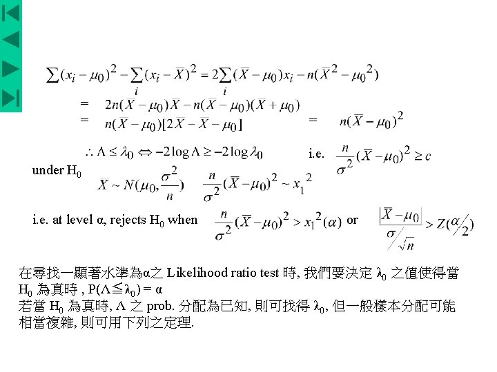
9. 7 The Poisson Dispersion Test The likelihood ratio test及Pearson’s chi-square test 是在未對 alternative hypothesis 作任何假設下得到的. 若我們對 alternative hyp. 有些了解, power一般 會比較好. 以下討論 Poisson dist. 之檢定. 樹葉上的昆蟲數: 當葉子大小不同時, 且採自於不同的植物時, 可能各個 counts 之 rates λ 並不同. 昆蟲孵出時通常都是一群一群, 所以不滿足 independence 之假設. 給定 counts x 1, …, xn H 0 : xi 來自 P(λ) v. s. H 1 : xi 來自 P (λi ) under H 0, . under Ω. M. C. E. of λi 為 xi

利用 Taylor Series argument 可得近似之對等型式. ∵under Ω = W 0∪W 1 有 n 個 free parameters ∴ dimΩ = n under W 0 dim W 0 = 1 ∴ degree of freedom dimΩ-dim W 0 為 n-1.

對 Poisson dist. 而言, mean 和 variance 是一致的. 而對 H 1 而言, variance 是大於 mean. 故此檢定常被稱為 the Poisson dispersion test. 此檢定 alternatives 一若相對於 Poisson dist. 為 overdispersed. 如 negative binomial dist. The ratio 有時用來測量群聚的程度. (在沒有足夠數據, 使得在好幾個 cells 中無法 累積有相當的數據, 以致無法使用 Pearson’s chi-square test 時, 即用Poisson disp. test) (每個 cell 中至少要有5個 obs. 才會使得 Pearson chi-square 中的檢定統計 量接近一 的分佈) Ex. A. (石綿纖維之例) 國家標準局. 石綿纖維在 23方格上之 counts 是否可用 Poisson dist. 來fit. 用 Poisson dispersion test. or likelihood ratio test d. f. = 23 – 1 = 22 p-value 大約為 0. 21 ∴證據不足以拒絕 H 0, 但因樣本小(23個 obs. ), power 可能較低.

Ex. B. (細菌塊) 牛奶中之細菌塊是否可用 Poisson = 4. 59 under H 0 T~ 由中央極限定理. ∴Poisson model fails to fit the data.

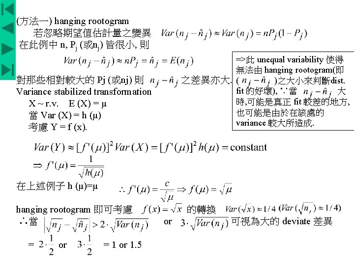
(方法二) hanging chi-gram (= components of Pearson’s chi-square statistics) ( ) ∴此方法亦 stabilize the variance of nj

Ex. A：前述之probability plot之方法應用在Michelson之光 速測定實驗數據，由 1897年 6月5日至 7月2日，將原始值 減去 299000後之100個數據如下(data from Stigler 1977)： Fig. 9. 4

Fig. 9. 5 Fig. 9. 6 Fig. 9. 7 precipitation

Ex. D：血清中含鉀的成分 deviation in the right tail are apparent