Lesson 14 1 Test for Goodness of Fit

Lesson 14 - 1 Test for Goodness of Fit One-Way Tables

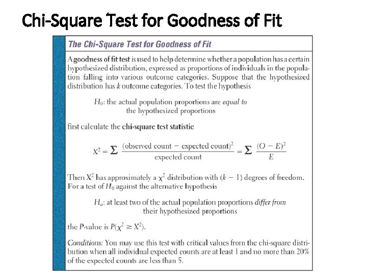
Knowledge Objectives • Describe the situation for which the chi-square test for goodness of fit is appropriate • Define the χ2 statistic, and identify the number of degrees of freedom it is based on, for the χ2 goodness of fit test • List the conditions that need to be satisfied in order to conduct a test χ2 for goodness of fit • Identify three main properties of the chi-square density curve

Construction Objectives • Conduct a χ2 test for goodness of fit. • Use technology to conduct a χ2 test for goodness of fit. • If a χ2 statistic turns out to be significant, discuss how to determine which observations contribute the most to the total value.

Vocabulary • Goodness-of-fit test – an inferential procedure used to determine whether a categorical frequency distribution follows a claimed distribution. • Expected counts – probability of an outcome times the sample size for k mutually exclusive outcomes • One-way table – a table of k mutually exclusive observed values • Cells – one item in the one-way table

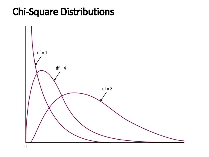
Chi-Square Distributions

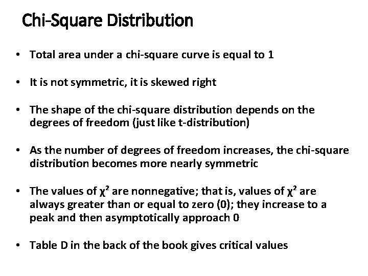
Chi-Square Distribution • Total area under a chi-square curve is equal to 1 • It is not symmetric, it is skewed right • The shape of the chi-square distribution depends on the degrees of freedom (just like t-distribution) • As the number of degrees of freedom increases, the chi-square distribution becomes more nearly symmetric • The values of χ² are nonnegative; that is, values of χ² are always greater than or equal to zero (0); they increase to a peak and then asymptotically approach 0 • Table D in the back of the book gives critical values

Chi-Square Test for Goodness of Fit

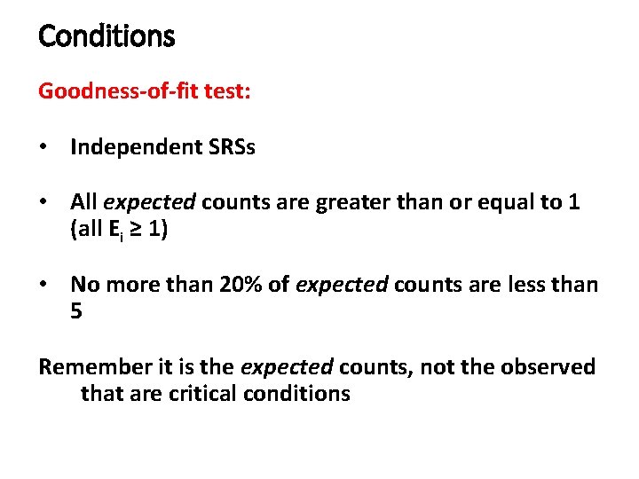
Conditions Goodness-of-fit test: • Independent SRSs • All expected counts are greater than or equal to 1 (all Ei ≥ 1) • No more than 20% of expected counts are less than 5 Remember it is the expected counts, not the observed that are critical conditions

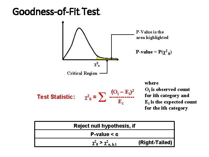
Goodness-of-Fit Test P-Value is the area highlighted P-value = P(χ2 0) χ2α Critical Region Test Statistic: χ2 0 = Σ (Oi – Ei)2 ------Ei where Oi is observed count for ith category and Ei is the expected count for the ith category Reject null hypothesis, if P-value < α χ20 > χ2α, k-1 (Right-Tailed)

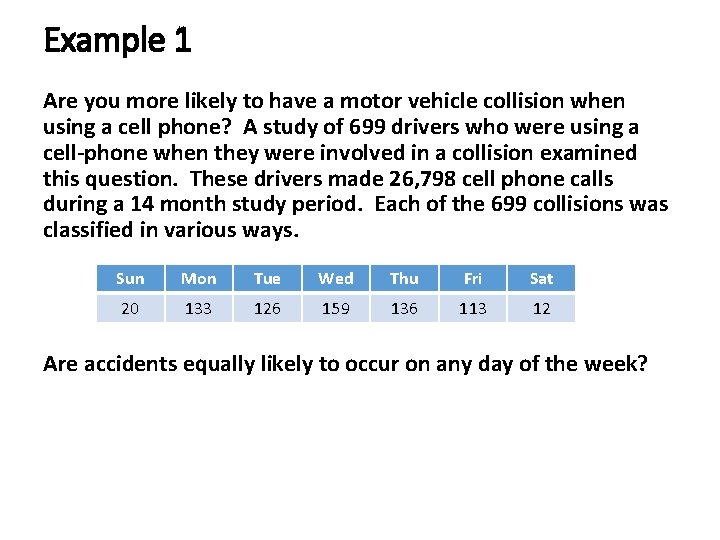
Example 1 Are you more likely to have a motor vehicle collision when using a cell phone? A study of 699 drivers who were using a cell-phone when they were involved in a collision examined this question. These drivers made 26, 798 cell phone calls during a 14 month study period. Each of the 699 collisions was classified in various ways. Sun Mon Tue Wed Thu Fri Sat 20 133 126 159 136 113 12 Are accidents equally likely to occur on any day of the week?

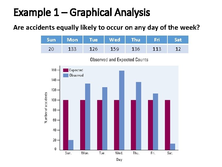
Example 1 – Graphical Analysis Are accidents equally likely to occur on any day of the week? Sun Mon Tue Wed Thu Fri Sat 20 133 126 159 136 113 12

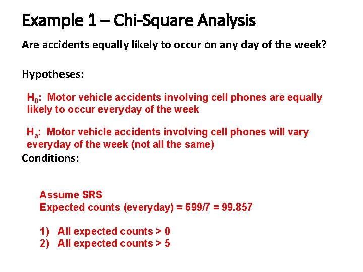
Example 1 – Chi-Square Analysis Are accidents equally likely to occur on any day of the week? Hypotheses: H 0: Motor vehicle accidents involving cell phones are equally likely to occur everyday of the week Ha: Motor vehicle accidents involving cell phones will vary everyday of the week (not all the same) Conditions: Assume SRS Expected counts (everyday) = 699/7 = 99. 857 1) All expected counts > 0 2) All expected counts > 5

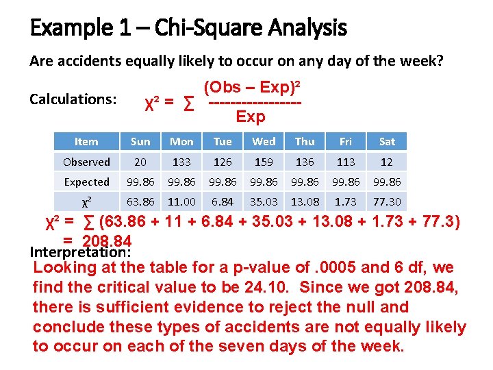
Example 1 – Chi-Square Analysis Are accidents equally likely to occur on any day of the week? Calculations: (Obs – Exp)² χ² = ∑ --------Exp Item Sun Mon Tue Wed Thu Fri Sat Observed 20 133 126 159 136 113 12 Expected 99. 86 99. 86 χ² 63. 86 11. 00 6. 84 35. 03 13. 08 1. 73 77. 30 χ² = ∑ (63. 86 + 11 + 6. 84 + 35. 03 + 13. 08 + 1. 73 + 77. 3) = 208. 84 Interpretation: Looking at the table for a p-value of. 0005 and 6 df, we find the critical value to be 24. 10. Since we got 208. 84, there is sufficient evidence to reject the null and conclude these types of accidents are not equally likely to occur on each of the seven days of the week.

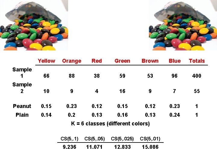
Example 2 Yellow Orange Red Green Brown Blue Totals Sample 1 66 88 38 59 53 96 400 Sample 2 10 9 4 16 9 7 55 Peanut 0. 15 0. 23 0. 12 0. 15 0. 12 0. 23 1 Plain 0. 14 0. 2 0. 13 0. 16 0. 13 0. 24 1 K = 6 classes (different colors) CS(5, . 1) CS(5, . 05) CS(5, . 025) CS(5, . 01) 9. 236 11. 071 12. 833 15. 086

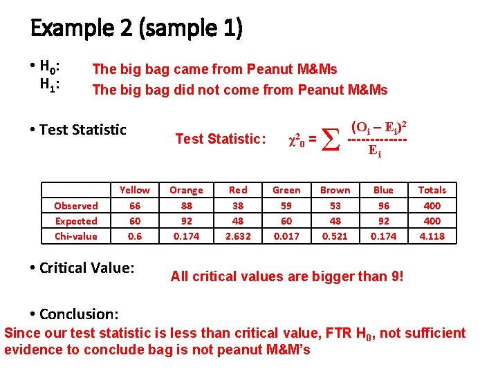
Example 2 (sample 1) • H 0: H 1: The big bag came from Peanut M&Ms The big bag did not come from Peanut M&Ms • Test Statistic Observed Expected Chi-value Yellow 66 60 0. 6 • Critical Value: Test Statistic: Orange 88 92 0. 174 Red 38 48 2. 632 χ2 0 = Green 59 60 0. 017 Σ (Oi – Ei)2 ------Ei Brown 53 48 0. 521 Blue 96 92 0. 174 Totals 400 4. 118 All critical values are bigger than 9! • Conclusion: Since our test statistic is less than critical value, FTR H 0, not sufficient evidence to conclude bag is not peanut M&M’s

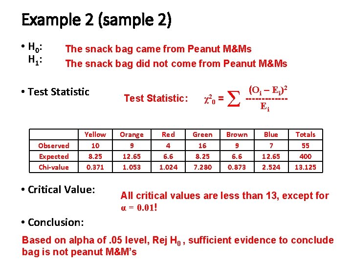
Example 2 (sample 2) • H 0: H 1: The snack bag came from Peanut M&Ms The snack bag did not come from Peanut M&Ms • Test Statistic Observed Expected Chi-value Yellow 10 8. 25 0. 371 • Critical Value: Test Statistic: Orange 9 12. 65 1. 053 Red 4 6. 6 1. 024 χ2 0 = Green 16 8. 25 7. 280 Σ (Oi – Ei)2 ------Ei Brown 9 6. 6 0. 873 Blue 7 12. 65 2. 524 Totals 55 400 13. 125 All critical values are less than 13, except for α = 0. 01! • Conclusion: Based on alpha of. 05 level, Rej H 0 , sufficient evidence to conclude bag is not peanut M&M’s

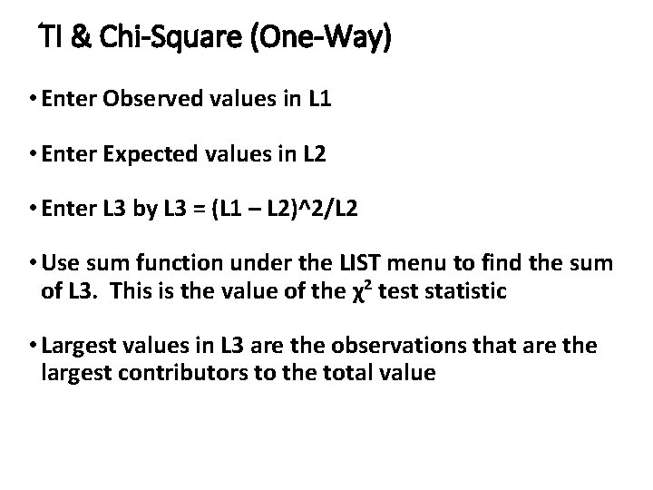
TI & Chi-Square (One-Way) • Enter Observed values in L 1 • Enter Expected values in L 2 • Enter L 3 by L 3 = (L 1 – L 2)^2/L 2 • Use sum function under the LIST menu to find the sum of L 3. This is the value of the χ² test statistic • Largest values in L 3 are the observations that are the largest contributors to the total value

Summary and Homework • Summary • Goodness-of-fit tests apply to situations where there a series of independent trials, and each trial has 3 or more possible outcomes • The test statistic to be used combines all of the outcomes and all of the expected counts • The test statistic has approximately a chi-square distribution • Pg. 843 gives step by step calculator directions • Homework • 14. 1, 7, 8