F TEST OF GOODNESS OF FIT In an


- Slides: 42
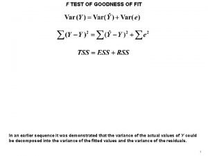
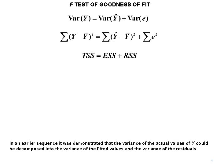
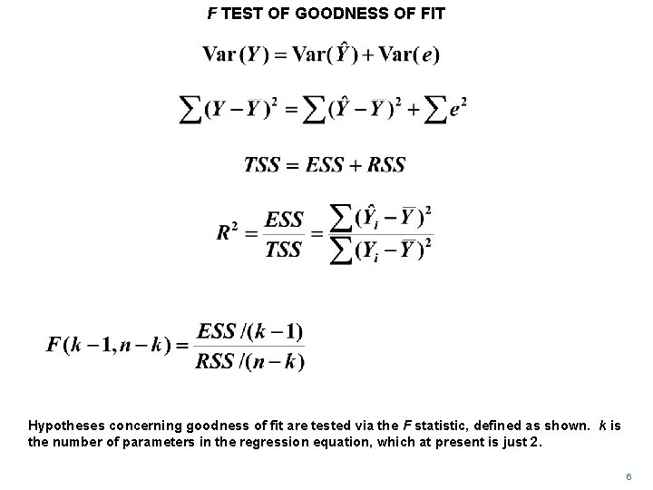
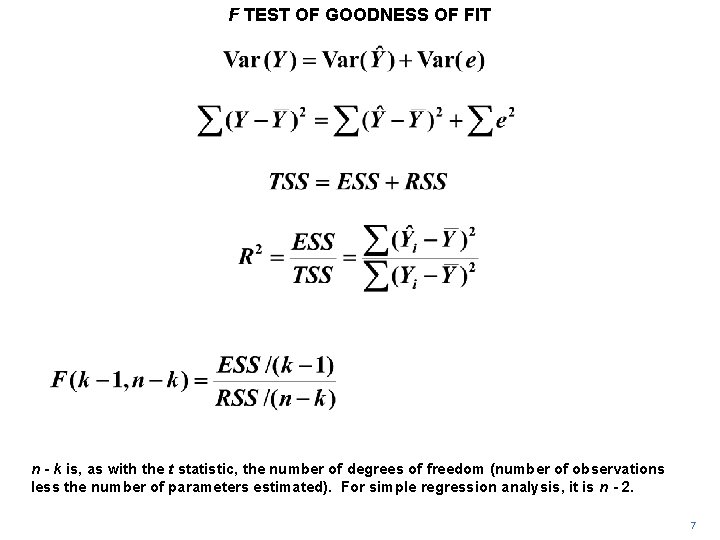
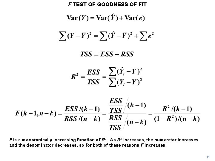
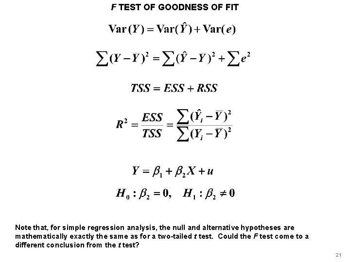
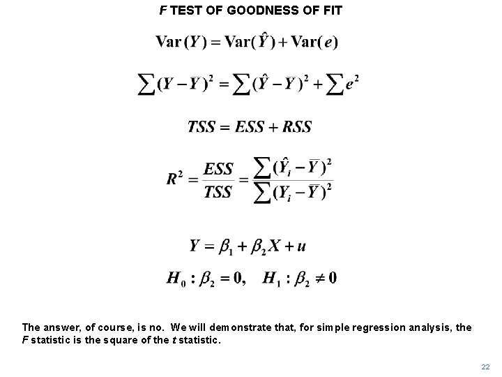
F TEST OF GOODNESS OF FIT In an earlier sequence it was demonstrated that the variance of the actual values of Y could be decomposed into the variance of the fitted values and the variance of the residuals. 1
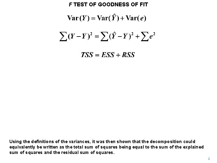
F TEST OF GOODNESS OF FIT Using the definitions of the variances, it was then shown that the decomposition could equivalently be written as the total sum of squares being equal to the sum of the explained sum of squares and the residual sum of squares. 2
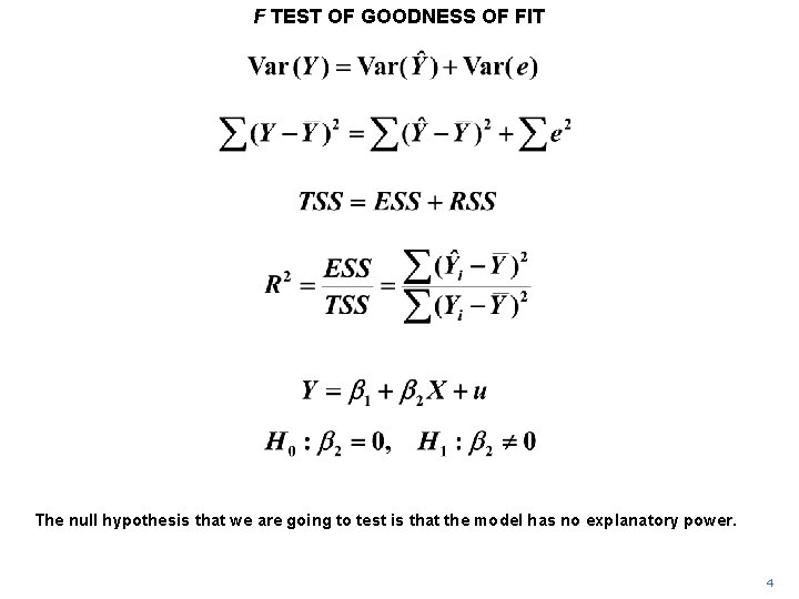
F TEST OF GOODNESS OF FIT R 2, the usual measure of goodness of fit, was then defined to be the ratio of the explained sum of squares to the total sum of squares. 3
F TEST OF GOODNESS OF FIT The null hypothesis that we are going to test is that the model has no explanatory power. 4
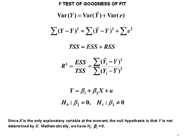
F TEST OF GOODNESS OF FIT Since X is the only explanatory variable at the moment, the null hypothesis is that Y is not determined by X. Mathematically, we have H 0: b 2 = 0. 5
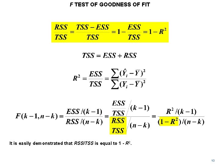
F TEST OF GOODNESS OF FIT Hypotheses concerning goodness of fit are tested via the F statistic, defined as shown. k is the number of parameters in the regression equation, which at present is just 2. 6
F TEST OF GOODNESS OF FIT n - k is, as with the t statistic, the number of degrees of freedom (number of observations less the number of parameters estimated). For simple regression analysis, it is n - 2. 7
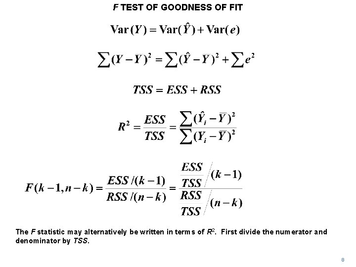
F TEST OF GOODNESS OF FIT The F statistic may alternatively be written in terms of R 2. First divide the numerator and denominator by TSS. 8
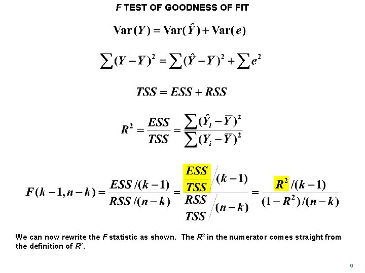
F TEST OF GOODNESS OF FIT We can now rewrite the F statistic as shown. The R 2 in the numerator comes straight from the definition of R 2. 9
F TEST OF GOODNESS OF FIT It is easily demonstrated that RSS/TSS is equal to 1 - R 2. 10
F TEST OF GOODNESS OF FIT F is a monotonically increasing function of R 2. As R 2 increases, the numerator increases and the denominator decreases, so for both of these reasons F increases. 11
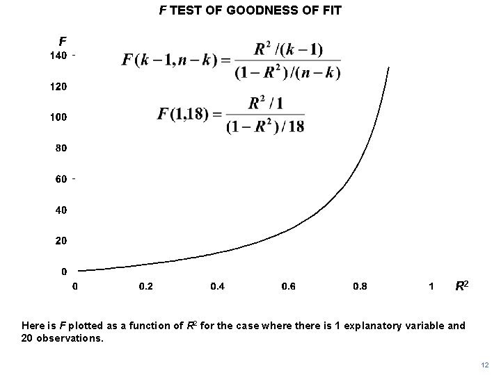
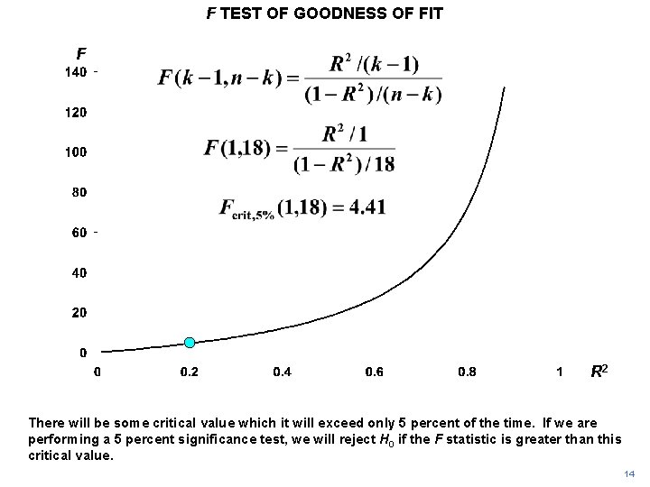
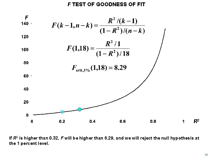
F TEST OF GOODNESS OF FIT F R 2 Here is F plotted as a function of R 2 for the case where there is 1 explanatory variable and 20 observations. 12
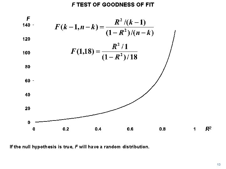
F TEST OF GOODNESS OF FIT F R 2 If the null hypothesis is true, F will have a random distribution. 13
F TEST OF GOODNESS OF FIT F R 2 There will be some critical value which it will exceed only 5 percent of the time. If we are performing a 5 percent significance test, we will reject H 0 if the F statistic is greater than this critical value. 14
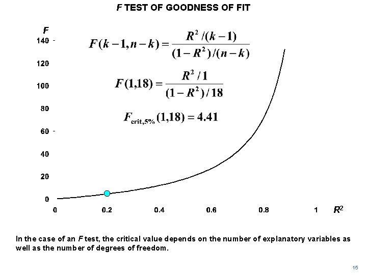
F TEST OF GOODNESS OF FIT F R 2 In the case of an F test, the critical value depends on the number of explanatory variables as well as the number of degrees of freedom. 15
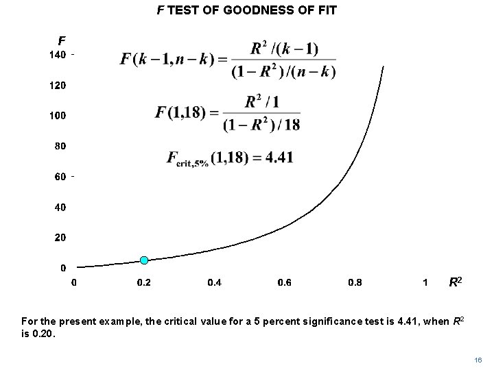
F TEST OF GOODNESS OF FIT F R 2 For the present example, the critical value for a 5 percent significance test is 4. 41, when R 2 is 0. 20. 16
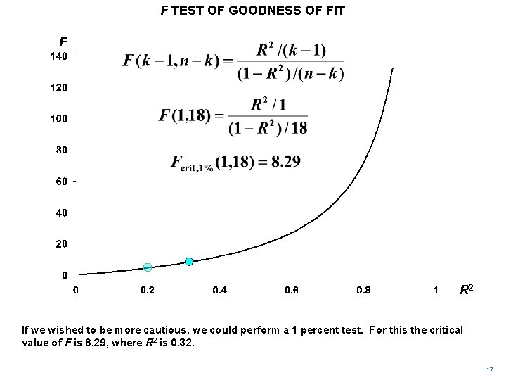
F TEST OF GOODNESS OF FIT F R 2 If we wished to be more cautious, we could perform a 1 percent test. For this the critical value of F is 8. 29, where R 2 is 0. 32. 17
F TEST OF GOODNESS OF FIT F R 2 If R 2 is higher than 0. 32, F will be higher than 8. 29, and we will reject the null hypothesis at the 1 percent level. 18
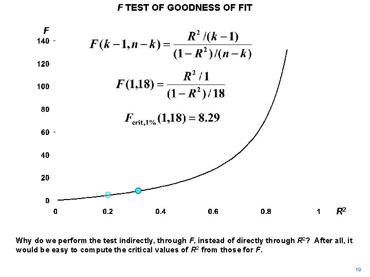
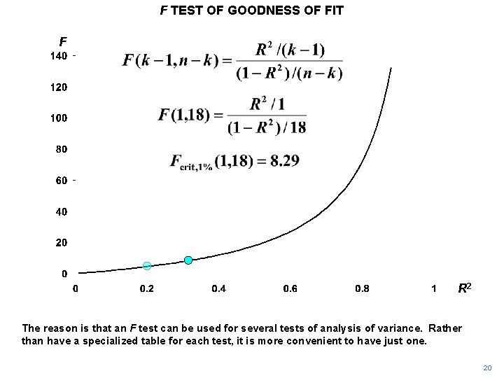
F TEST OF GOODNESS OF FIT F R 2 Why do we perform the test indirectly, through F, instead of directly through R 2? After all, it would be easy to compute the critical values of R 2 from those for F. 19
F TEST OF GOODNESS OF FIT F R 2 The reason is that an F test can be used for several tests of analysis of variance. Rather than have a specialized table for each test, it is more convenient to have just one. 20
F TEST OF GOODNESS OF FIT Note that, for simple regression analysis, the null and alternative hypotheses are mathematically exactly the same as for a two-tailed t test. Could the F test come to a different conclusion from the t test? 21
F TEST OF GOODNESS OF FIT The answer, of course, is no. We will demonstrate that, for simple regression analysis, the F statistic is the square of the t statistic. 22
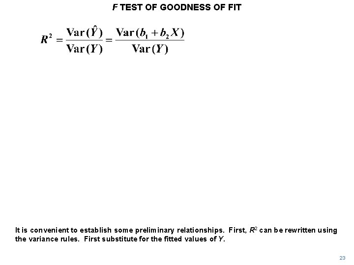
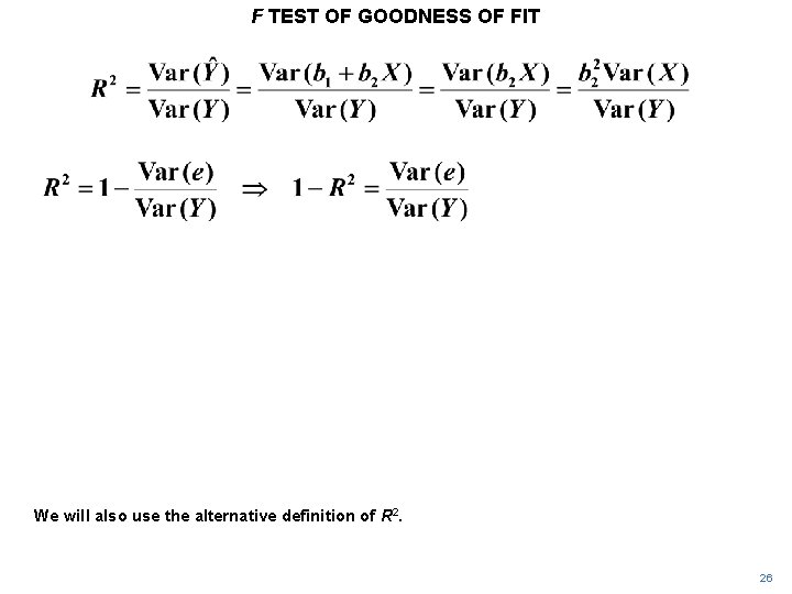
F TEST OF GOODNESS OF FIT It is convenient to establish some preliminary relationships. First, R 2 can be rewritten using the variance rules. First substitute for the fitted values of Y. 23
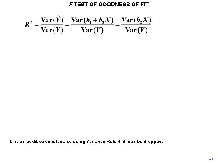
F TEST OF GOODNESS OF FIT b 1 is an additive constant, so using Variance Rule 4, it may be dropped. 24
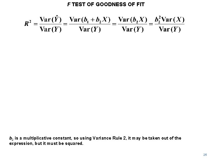
F TEST OF GOODNESS OF FIT b 2 is a multiplicative constant, so using Variance Rule 2, it may be taken out of the expression, but it must be squared. 25
F TEST OF GOODNESS OF FIT We will also use the alternative definition of R 2. 26
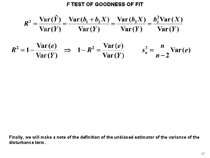
F TEST OF GOODNESS OF FIT Finally, we will make a note of the definition of the unbiased estimator of the variance of the disturbance term. 27
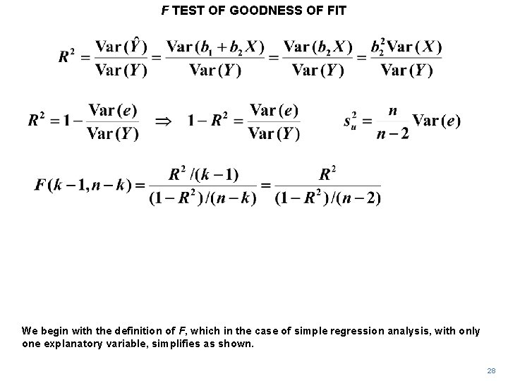
F TEST OF GOODNESS OF FIT We begin with the definition of F, which in the case of simple regression analysis, with only one explanatory variable, simplifies as shown. 28
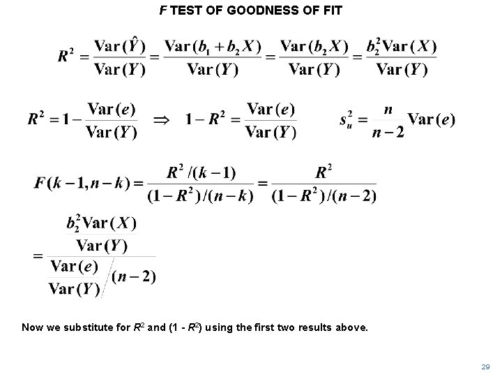
F TEST OF GOODNESS OF FIT Now we substitute for R 2 and (1 - R 2) using the first two results above. 29
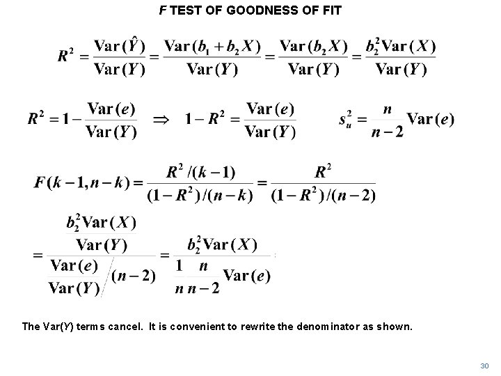
F TEST OF GOODNESS OF FIT The Var(Y) terms cancel. It is convenient to rewrite the denominator as shown. 30
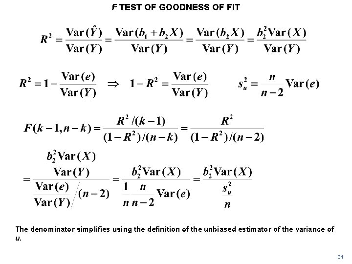
F TEST OF GOODNESS OF FIT The denominator simplifies using the definition of the unbiased estimator of the variance of u. 31
F TEST OF GOODNESS OF FIT Hence we obtain b 22 divided by the square of the standard error of b 2. This is the t statistic, squared. 32
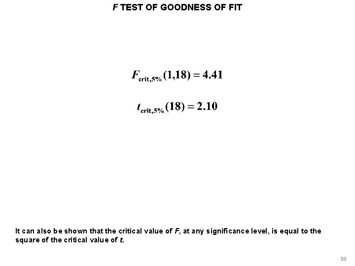
F TEST OF GOODNESS OF FIT It can also be shown that the critical value of F, at any significance level, is equal to the square of the critical value of t. 33
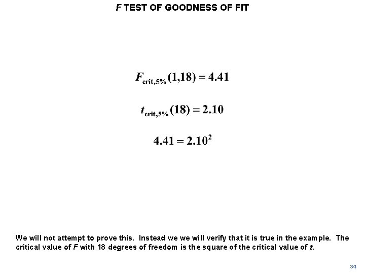
F TEST OF GOODNESS OF FIT We will not attempt to prove this. Instead we we will verify that it is true in the example. The critical value of F with 18 degrees of freedom is the square of the critical value of t. 34
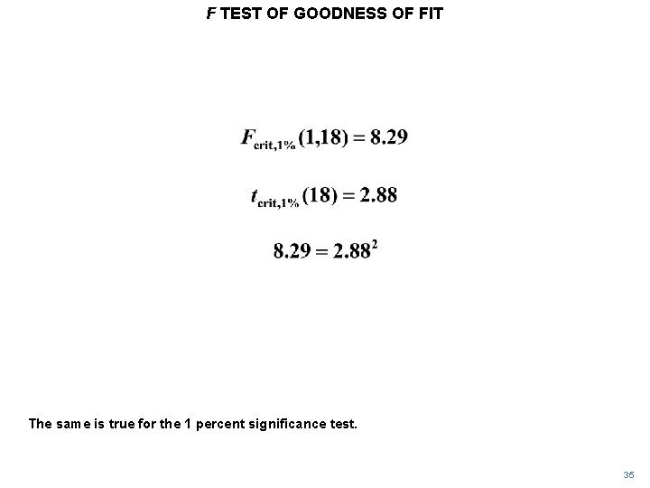
F TEST OF GOODNESS OF FIT The same is true for the 1 percent significance test. 35
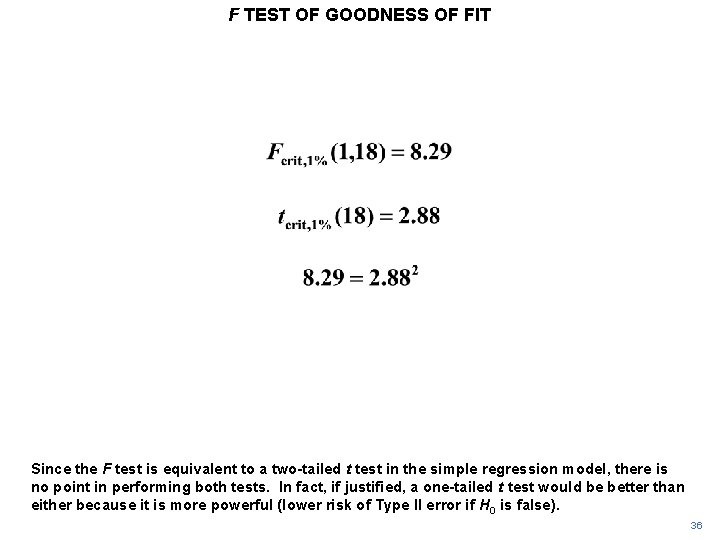
F TEST OF GOODNESS OF FIT Since the F test is equivalent to a two-tailed t test in the simple regression model, there is no point in performing both tests. In fact, if justified, a one-tailed t test would be better than either because it is more powerful (lower risk of Type II error if H 0 is false). 36
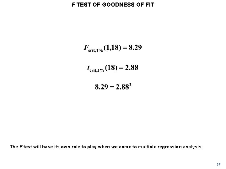
F TEST OF GOODNESS OF FIT The F test will have its own role to play when we come to multiple regression analysis. 37
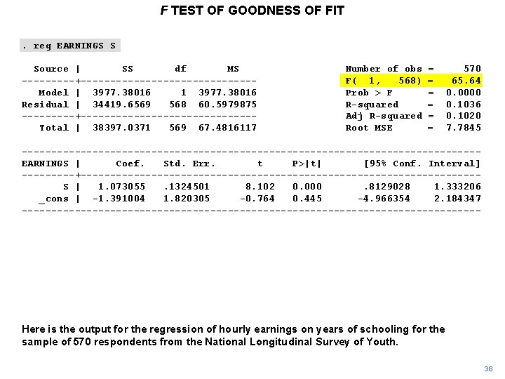
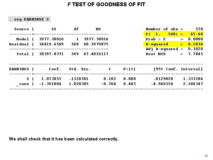
F TEST OF GOODNESS OF FIT. reg EARNINGS S Source | SS df MS -----+---------------Model | 3977. 38016 1 3977. 38016 Residual | 34419. 6569 568 60. 5979875 -----+---------------Total | 38397. 0371 569 67. 4816117 Number of obs F( 1, 568) Prob > F R-squared Adj R-squared Root MSE = = = 570 65. 64 0. 0000 0. 1036 0. 1020 7. 7845 ---------------------------------------EARNINGS | Coef. Std. Err. t P>|t| [95% Conf. Interval] -----+----------------------------------S | 1. 073055. 1324501 8. 102 0. 000. 8129028 1. 333206 _cons | -1. 391004 1. 820305 -0. 764 0. 445 -4. 966354 2. 184347 --------------------------------------- Here is the output for the regression of hourly earnings on years of schooling for the sample of 570 respondents from the National Longitudinal Survey of Youth. 38
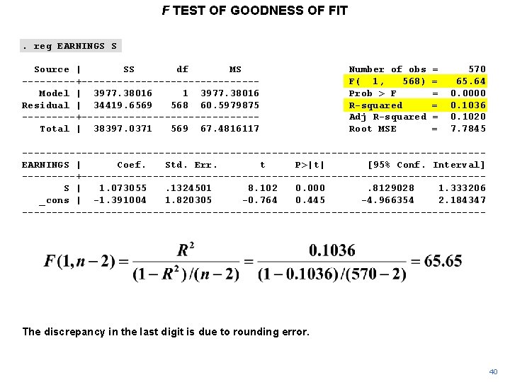
F TEST OF GOODNESS OF FIT. reg EARNINGS S Source | SS df MS -----+---------------Model | 3977. 38016 1 3977. 38016 Residual | 34419. 6569 568 60. 5979875 -----+---------------Total | 38397. 0371 569 67. 4816117 Number of obs F( 1, 568) Prob > F R-squared Adj R-squared Root MSE = = = 570 65. 64 0. 0000 0. 1036 0. 1020 7. 7845 ---------------------------------------EARNINGS | Coef. Std. Err. t P>|t| [95% Conf. Interval] -----+----------------------------------S | 1. 073055. 1324501 8. 102 0. 000. 8129028 1. 333206 _cons | -1. 391004 1. 820305 -0. 764 0. 445 -4. 966354 2. 184347 --------------------------------------- We shall check that it has been calculated correctly. 39
F TEST OF GOODNESS OF FIT. reg EARNINGS S Source | SS df MS -----+---------------Model | 3977. 38016 1 3977. 38016 Residual | 34419. 6569 568 60. 5979875 -----+---------------Total | 38397. 0371 569 67. 4816117 Number of obs F( 1, 568) Prob > F R-squared Adj R-squared Root MSE = = = 570 65. 64 0. 0000 0. 1036 0. 1020 7. 7845 ---------------------------------------EARNINGS | Coef. Std. Err. t P>|t| [95% Conf. Interval] -----+----------------------------------S | 1. 073055. 1324501 8. 102 0. 000. 8129028 1. 333206 _cons | -1. 391004 1. 820305 -0. 764 0. 445 -4. 966354 2. 184347 --------------------------------------- The discrepancy in the last digit is due to rounding error. 40
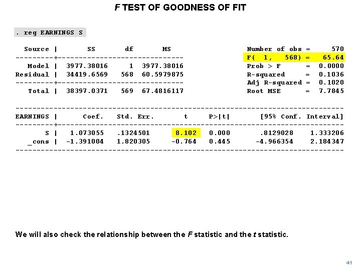
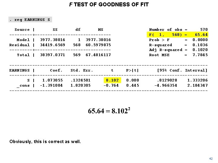
F TEST OF GOODNESS OF FIT. reg EARNINGS S Source | SS df MS -----+---------------Model | 3977. 38016 1 3977. 38016 Residual | 34419. 6569 568 60. 5979875 -----+---------------Total | 38397. 0371 569 67. 4816117 Number of obs F( 1, 568) Prob > F R-squared Adj R-squared Root MSE = = = 570 65. 64 0. 0000 0. 1036 0. 1020 7. 7845 ---------------------------------------EARNINGS | Coef. Std. Err. t P>|t| [95% Conf. Interval] -----+----------------------------------S | 1. 073055. 1324501 8. 102 0. 000. 8129028 1. 333206 _cons | -1. 391004 1. 820305 -0. 764 0. 445 -4. 966354 2. 184347 --------------------------------------- We will also check the relationship between the F statistic and the t statistic. 41
F TEST OF GOODNESS OF FIT. reg EARNINGS S Source | SS df MS -----+---------------Model | 3977. 38016 1 3977. 38016 Residual | 34419. 6569 568 60. 5979875 -----+---------------Total | 38397. 0371 569 67. 4816117 Number of obs F( 1, 568) Prob > F R-squared Adj R-squared Root MSE = = = 570 65. 64 0. 0000 0. 1036 0. 1020 7. 7845 ---------------------------------------EARNINGS | Coef. Std. Err. t P>|t| [95% Conf. Interval] -----+----------------------------------S | 1. 073055. 1324501 8. 102 0. 000. 8129028 1. 333206 _cons | -1. 391004 1. 820305 -0. 764 0. 445 -4. 966354 2. 184347 --------------------------------------- Obviously, this is correct as well. 42