Goodness of Fit Tests Chi 2 Test for

Goodness of Fit Tests Chi 2 Test for hypothesized distributions

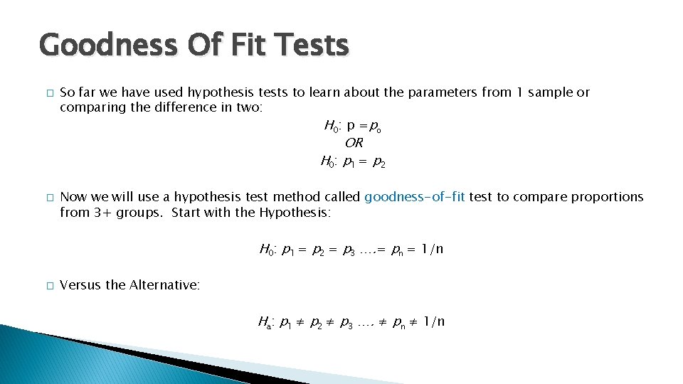
Goodness Of Fit Tests � So far we have used hypothesis tests to learn about the parameters from 1 sample or comparing the difference in two: H 0: p =po OR H 0: p 1 = p 2 � Now we will use a hypothesis test method called goodness-of-fit test to compare proportions from 3+ groups. Start with the Hypothesis: H 0: p 1 = p 2 = p 3 …. = pn = 1/n � Versus the Alternative: Ha: p 1 ≠ p 2 ≠ p 3 …. ≠ pn ≠ 1/n

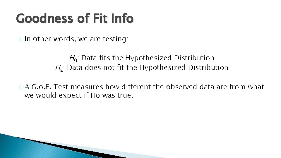
Goodness of Fit Info � In other words, we are testing: H 0: Data fits the Hypothesized Distribution Ha: Data does not fit the Hypothesized Distribution �A G. o. F. Test measures how different the observed data are from what we would expect if Ho was true.

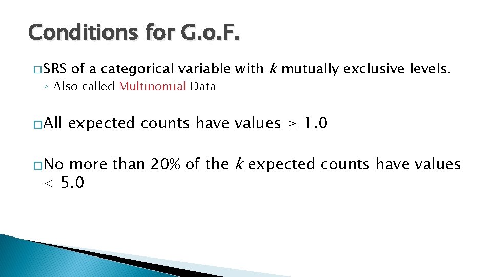
Conditions for G. o. F. � SRS of a categorical variable with k mutually exclusive levels. ◦ Also called Multinomial Data �All expected counts have values ≥ 1. 0 more than 20% of the k expected counts have values < 5. 0 �No

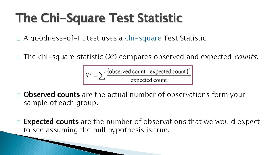
The Chi-Square Test Statistic � A goodness-of-fit test uses a chi-square Test Statistic � The chi-square statistic (X 2) compares observed and expected counts. � � Observed counts are the actual number of observations form your sample of each group. Expected counts are the number of observations that we would expect to see assuming the null hypothesis is true.

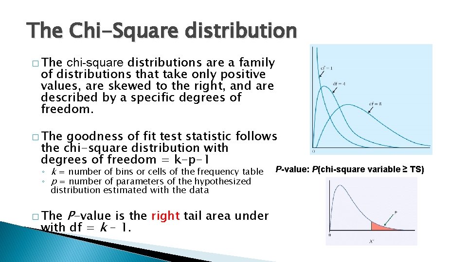
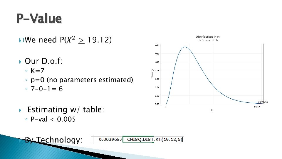
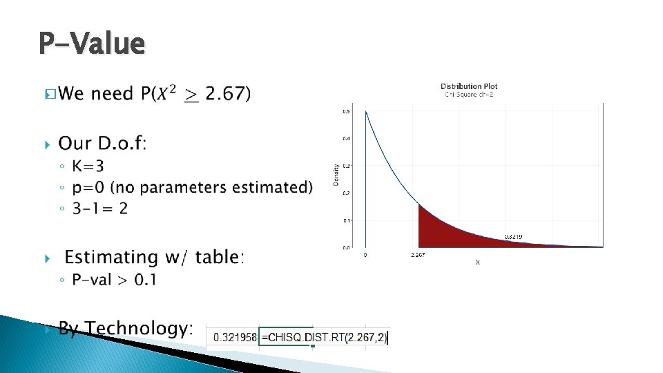
The Chi-Square distribution � The chi-square distributions are a family of distributions that take only positive values, are skewed to the right, and are described by a specific degrees of freedom. � The goodness of fit test statistic follows the chi-square distribution with degrees of freedom = k-p-1 ◦ k = number of bins or cells of the frequency table ◦ p = number of parameters of the hypothesized distribution estimated with the data P-value is the right tail area under with df = k – 1. � The P-value: P(chi-square variable ≥ TS)

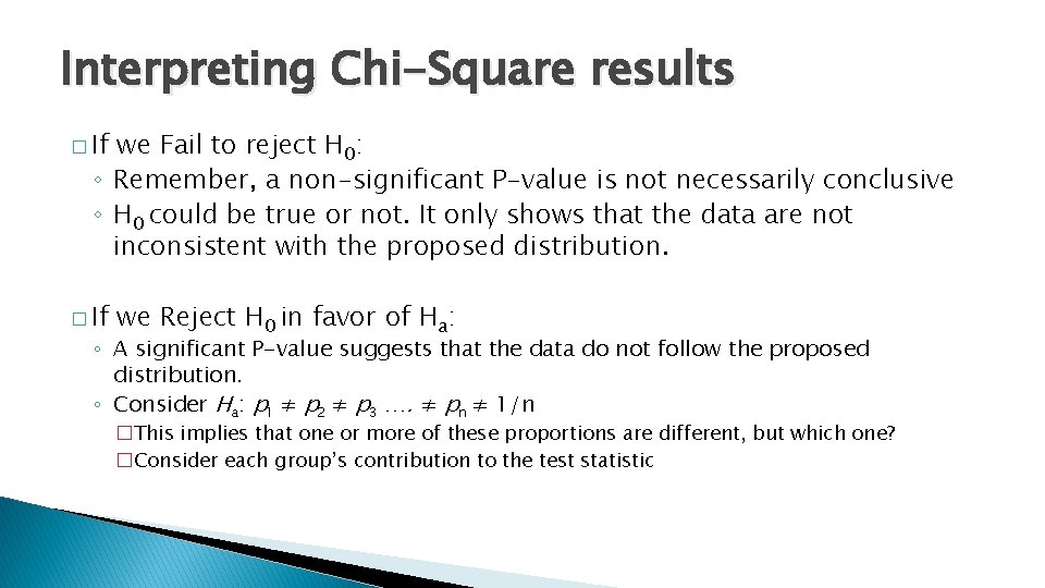
Interpreting Chi-Square results � If we Fail to reject H 0: ◦ Remember, a non-significant P-value is not necessarily conclusive ◦ H 0 could be true or not. It only shows that the data are not inconsistent with the proposed distribution. � If we Reject H 0 in favor of Ha: ◦ A significant P-value suggests that the data do not follow the proposed distribution. ◦ Consider Ha: p 1 ≠ p 2 ≠ p 3 …. ≠ pn ≠ 1/n �This implies that one or more of these proportions are different, but which one? �Consider each group’s contribution to the test statistic

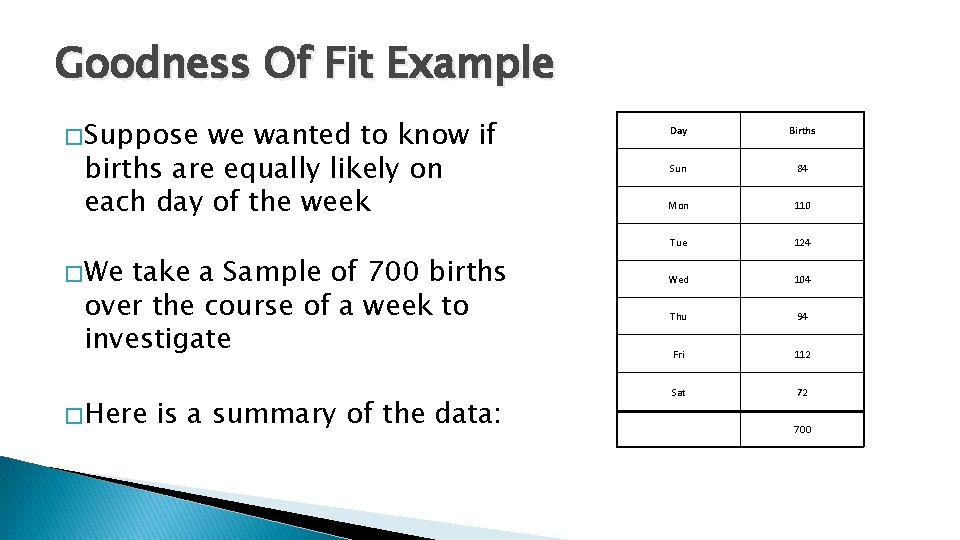
Goodness Of Fit Example � Suppose we wanted to know if births are equally likely on each day of the week � We take a Sample of 700 births over the course of a week to investigate � Here is a summary of the data: Day Births Sun 84 Mon 110 Tue 124 Wed 104 Thu 94 Fri 112 Sat 72 700

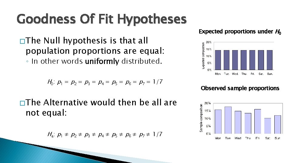
Goodness Of Fit Hypotheses � The Null hypothesis is that all population proportions are equal: Expected proportions under H 0 ◦ In other words uniformly distributed. H 0: p 1 = p 2 = p 3 = p 4 = p 5 = p 6 = p 7 = 1/7 � The Alternative would then be all are not equal: Ha: p 1 ≠ p 2 ≠ p 3 ≠ p 4 ≠ p 5 ≠ p 6 ≠ p 7 ≠ 1/7 Observed sample proportions

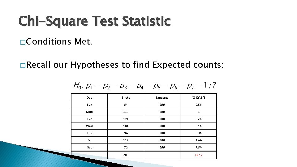
Chi-Square Test Statistic � Conditions � Recall Met. our Hypotheses to find Expected counts: H 0: p 1 = p 2 = p 3 = p 4 = p 5 = p 6 = p 7 = 1/7 Day Births Expected (O-E)^2/E Sun 84 100 2. 56 Mon 110 100 1 Tue 124 100 5. 76 Wed 104 100 0. 16 Thu 94 100 0. 36 Fri 112 100 1. 44 Sat 72 100 7. 84 700 19. 12

P-Value �

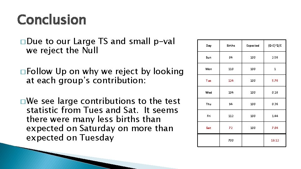
Conclusion � Due to our Large TS and small p-val we reject the Null � Follow Up on why we reject by looking at each group’s contribution: � We see large contributions to the test statistic from Tues and Sat. It seems there were many less births than expected on Saturday on more than expected on Tuesday Day Births Expected (O-E)^2/E Sun 84 100 2. 56 Mon 110 100 1 Tue 124 100 5. 76 Wed 104 100 0. 16 Thu 94 100 0. 36 Fri 112 100 1. 44 Sat 72 100 7. 84 700 19. 12

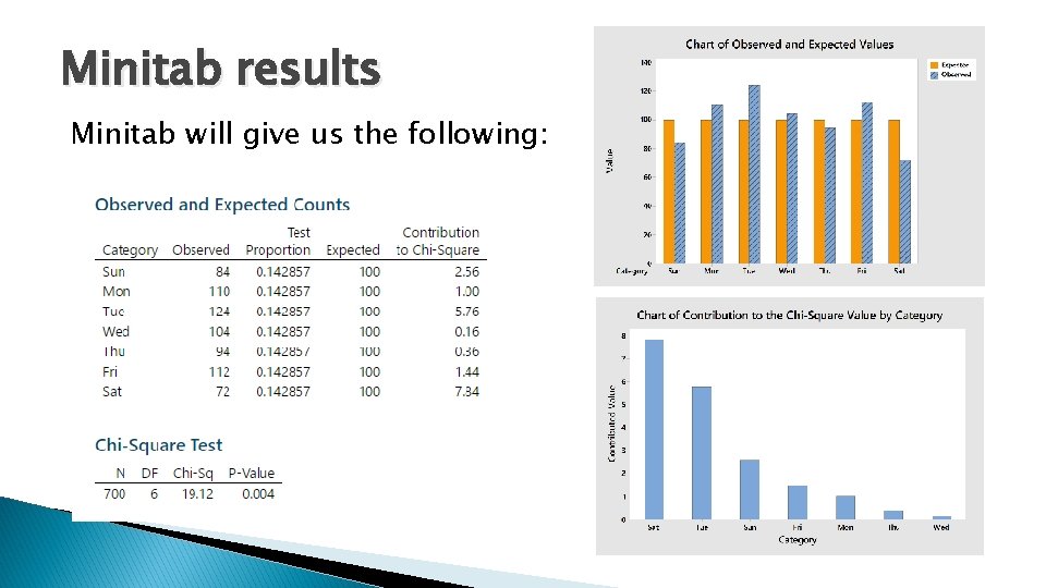
G. o. F. test in Minitab � Go to Stat -> Tables -> G. o. F (one variable) � Tell Minitab if you have frequencies (observed counts) or the raw Data (Categorical Data) � It will test equal proportions by default. If you have specific proportions you are testing (we will see this later) you must enter those into a separate column. � The Graphs provided can be useful, but not necessary

Minitab results Minitab will give us the following:

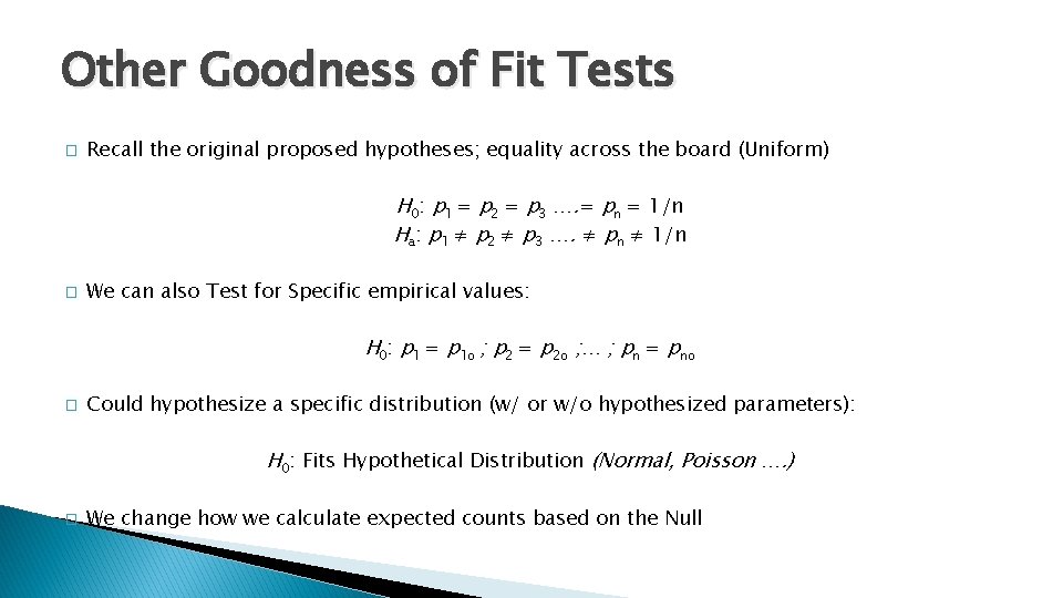
Other Goodness of Fit Tests � Recall the original proposed hypotheses; equality across the board (Uniform) H 0: p 1 = p 2 = p 3 …. = pn = 1/n Ha: p 1 ≠ p 2 ≠ p 3 …. ≠ pn ≠ 1/n � We can also Test for Specific empirical values: H 0: p 1 = p 1 o ; p 2 = p 2 o ; … ; pn = pno � Could hypothesize a specific distribution (w/ or w/o hypothesized parameters): H 0: Fits Hypothetical Distribution (Normal, Poisson …. ) � We change how we calculate expected counts based on the Null

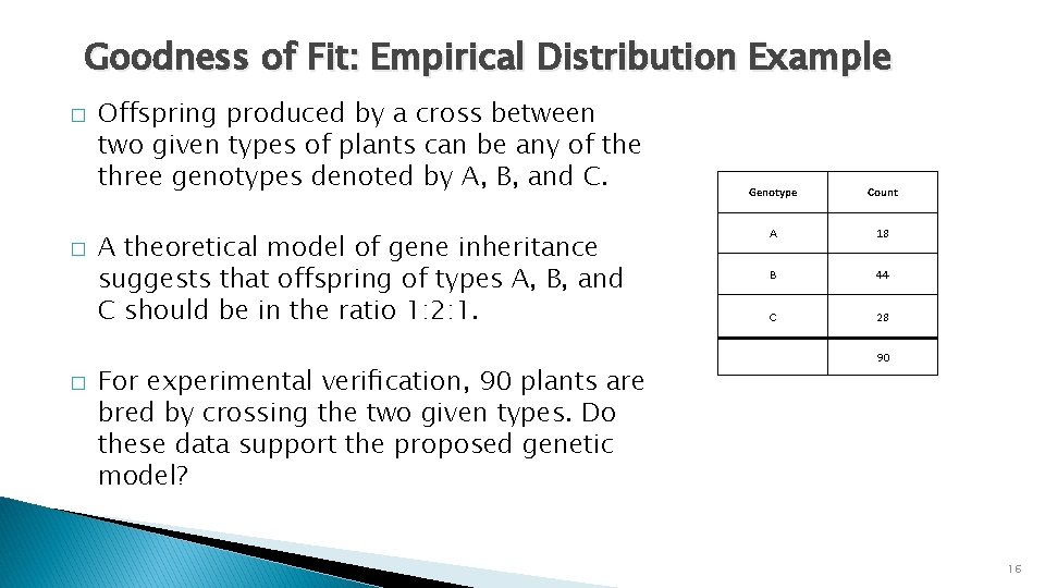
Goodness of Fit: Empirical Distribution Example � � � Offspring produced by a cross between two given types of plants can be any of the three genotypes denoted by A, B, and C. A theoretical model of gene inheritance suggests that offspring of types A, B, and C should be in the ratio 1: 2: 1. For experimental verification, 90 plants are bred by crossing the two given types. Do these data support the proposed genetic model? Genotype Count A 18 B 44 C 28 90 16

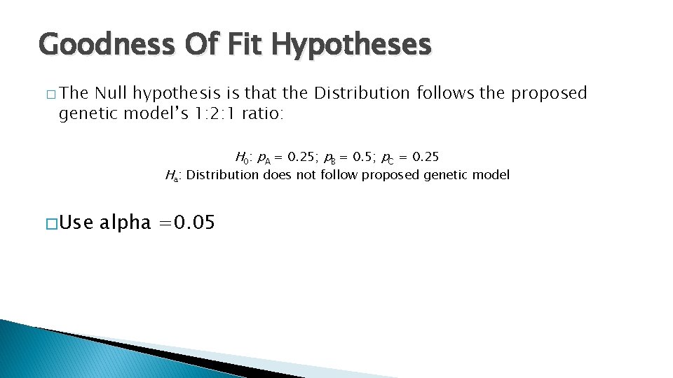
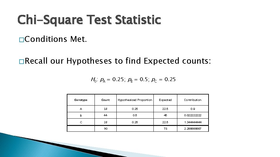
Goodness Of Fit Hypotheses � The Null hypothesis is that the Distribution follows the proposed genetic model’s 1: 2: 1 ratio: H 0: p. A = 0. 25; p. B = 0. 5; p. C = 0. 25 Ha: Distribution does not follow proposed genetic model � Use alpha =0. 05

Chi-Square Test Statistic � Conditions � Recall Met. our Hypotheses to find Expected counts: H 0: p. A = 0. 25; p. B = 0. 5; p. C = 0. 25 Genotype Count Hypothesized Proportion Expected Contribution A 18 0. 25 22. 5 0. 9 B 44 0. 5 45 0. 02222 C 28 0. 25 22. 5 1. 34444 90 TS 2. 266666667

P-Value �

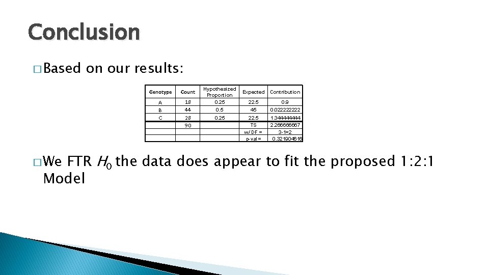
Conclusion � Based on our results: Genotype Count A B 18 44 28 C 90 Hypothesized Proportion 0. 25 Expected Contribution 22. 5 45 0. 9 0. 02222 22. 5 TS w/ DF = p-val = 1. 34444 2. 266666667 3 -1=2 0. 321904616 FTR H 0 the data does appear to fit the proposed 1: 2: 1 Model � We

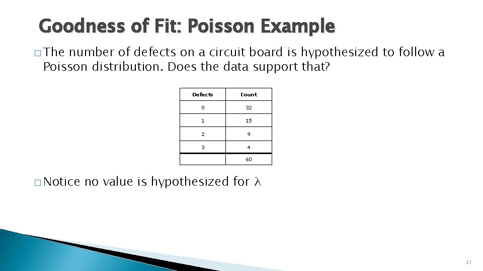
Goodness of Fit: Poisson Example � The number of defects on a circuit board is hypothesized to follow a Poisson distribution. Does the data support that? � Notice Defects Count 0 32 1 15 2 9 3 4 60 no value is hypothesized for λ 21

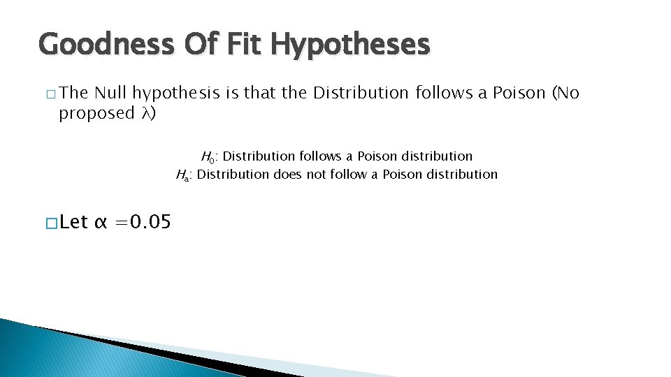
Goodness Of Fit Hypotheses � The Null hypothesis is that the Distribution follows a Poison (No proposed λ) H 0: Distribution follows a Poison distribution Ha: Distribution does not follow a Poison distribution � Let α =0. 05

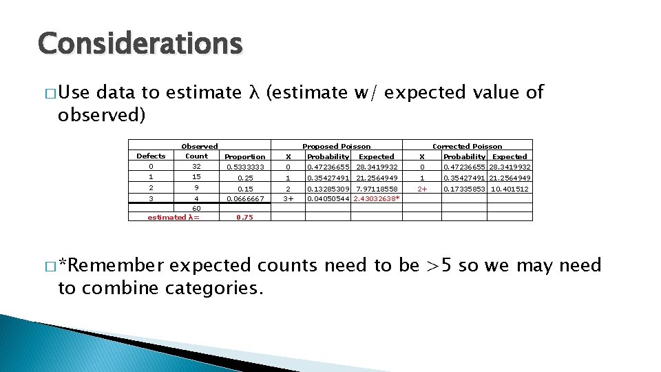
Considerations � Use data to estimate λ (estimate w/ expected value of observed) Defects 0 1 2 Observed Count Proportion 32 0. 5333333 15 0. 25 9 3 4 60 estimated λ= � *Remember 0. 15 0. 0666667 0. 75 X 0 Proposed Poisson Probability Expected 0. 47236655 28. 3419932 X 0 Corrected Poisson Probability Expected 0. 47236655 28. 3419932 1 0. 35427491 21. 2564949 2+ 0. 17335853 10. 401512 2 3+ 0. 13285309 7. 97118558 0. 04050544 2. 43032638* expected counts need to be >5 so we may need to combine categories.

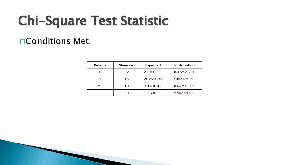
Chi-Square Test Statistic � Conditions Met. Defects Observed Expected Contribution 0 32 28. 3419932 0. 472126781 1 15 21. 2564949 1. 841494956 2+ 13 10. 401512 0. 649149865 60 60 2. 962771602

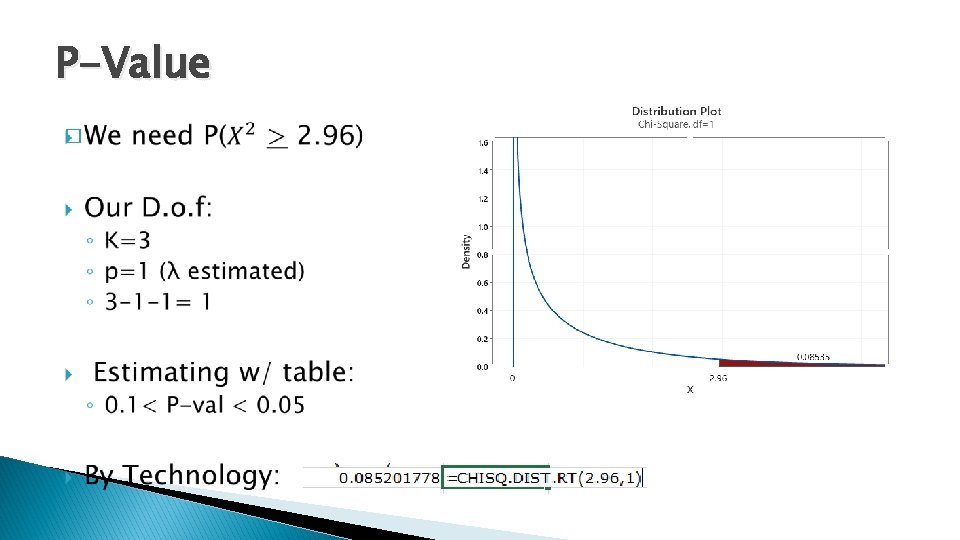
P-Value �

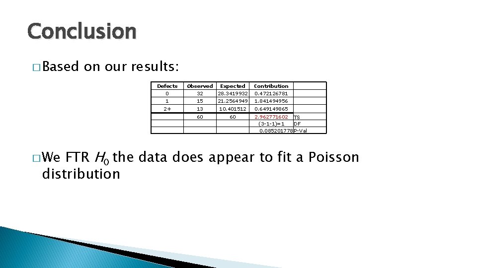
Conclusion � Based on our results: Defects 0 Observed Expected 32 28. 3419932 Contribution 0. 472126781 1 15 21. 2564949 1. 841494956 2+ 13 10. 401512 0. 649149865 60 60 2. 962771602 TS (3 -1 -1)=1 DF 0. 085201778 P-Val FTR H 0 the data does appear to fit a Poisson distribution � We