Bayesian MultilevelLongitudinal Models Using Stata Chuck Huber Ph

Bayesian Multilevel/Longitudinal Models Using Stata Chuck Huber, Ph. D Stata. Corp chuber@stata. com University of Illinois at Urbana-Champaign October 11, 2016

Outline • • • Introduction to Multilevel Models Introduction to Longitudinal Models Introduction to Bayesian Analysis Bayesian Multilevel Models Bayesian Longitudinal Models

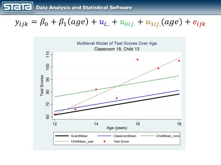
The Simulated Dataset • This dataset contains repeated measurements of test scores on children from age 12 -18 • The children are nested within classroom (admittedly not very realistic).

The Simulated Dataset

The Simulated Dataset

The Simulated Dataset

The Simulated Dataset

The Simulated Dataset

Outline • • • Introduction to Multilevel Models Introduction to Longitudinal Models Introduction to Bayesian Analysis Bayesian Multilevel Models Bayesian Longitudinal Models

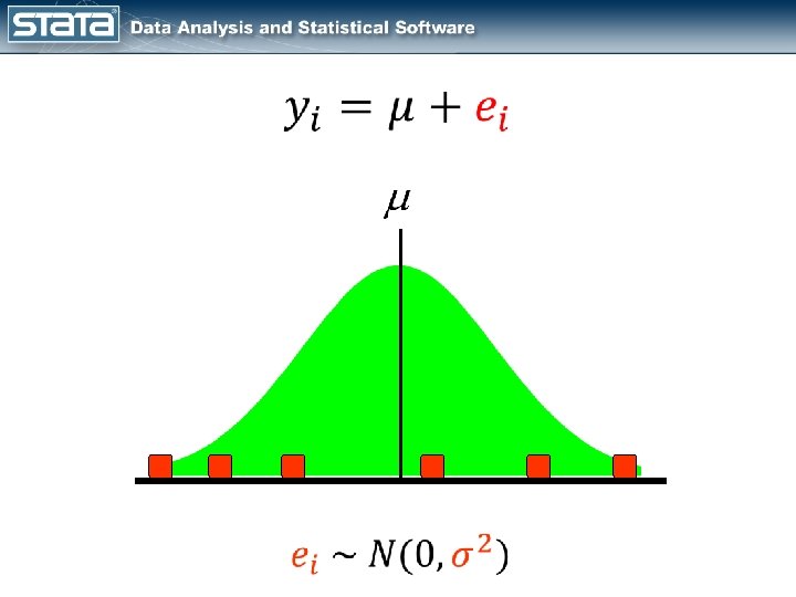
Single Level Models yi = y. Child We assume that observations of all children are independent of each other

Single Level Models

Single Level Models Observed Fixed Random

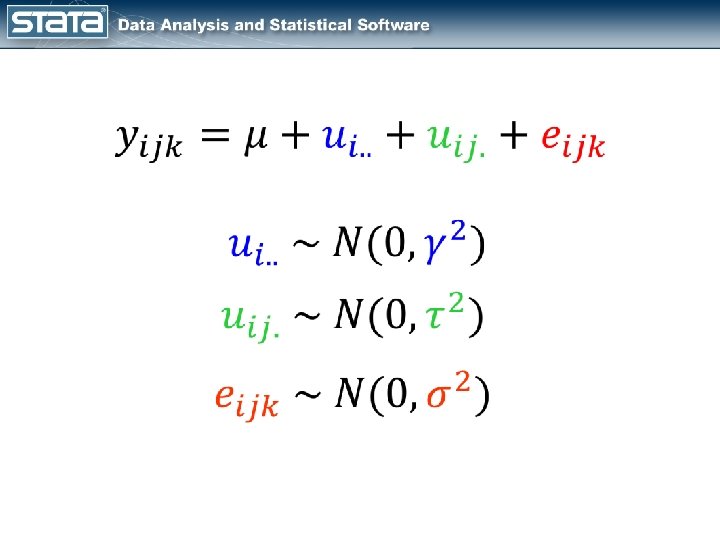
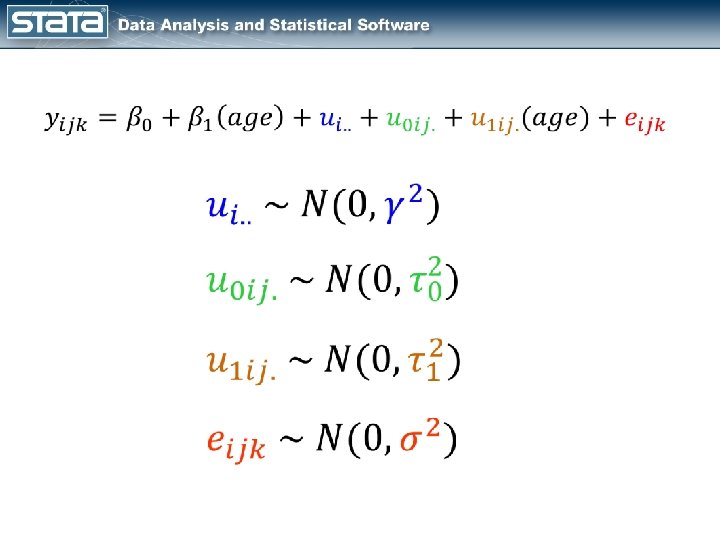
Three Level Models Classroom Child Observations Repeated observations within children from the same classroom may be correlated

Three Level Models Repeated observations within child will vary about each child’s mean.

Three Level Models Children’s means from the same classroom will vary about their classroom mean.

Three Level Models Classroom means will vary about the grand mean.

Three Level Models Level 3 Level 2 Level 1 We can refer to the nesting structure in terms of “Levels”…

i j k yijk = yclassroom, child, observation

Three Level Models Observed Fixed Random

Three Level Models

Three Level Models Observed Fixed Random

child mean classroom mean

child mean classroom mean
 18")
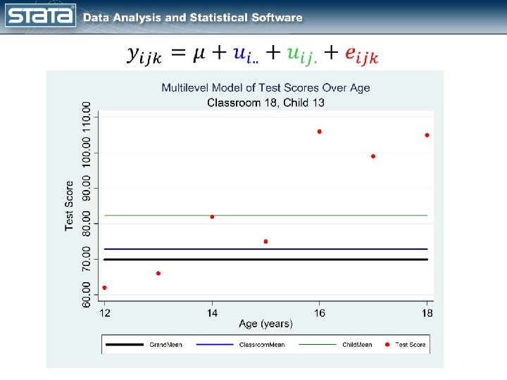
child mean classroom mean grand mean 10 Age (years) 18
 80")
Test Score child mean classroom mean grand mean 10 Age (years) 80

an Test Score child me ean m m o o r s clas 10 Age (years) 18
 Test Score")
xed sl i f ( n a e hild m ope) Test Score c 10 Age (years) 18
 d e x i f ( n a child me")
Test Score slope) d e x i f ( n a child me e) p o sl m o nd a r ( an e m d l i ch 10 Age (years) 18
 _ ( n a e child m e p slo")
Test Score cons) _ ( n a e child m e p slo dom n a ild r ch ns) (_co n a e m m classroo 10 Age (years) 18

How do we do this in Stata?
 50")
Test Score child mean classroom mean grand mean 30 Age (years) 50

. mixed Test. Score || classroom: || child: ---------------------------------------Test. Score | Coef. Std. Err. z P>|z| [95% Conf. Interval] -------+--------------------------------_cons | 69. 89633. 5487339 127. 38 0. 000 68. 82083 70. 97183 -----------------------------------------------------------------------------Random-effects Parameters | Estimate Std. Err. [95% Conf. Interval] ---------------+------------------------classroom: Identity | var(_cons) | 3. 475057 1. 909402 1. 183754 10. 20146 ---------------+------------------------child: Identity | var(_cons) | 69. 95854 4. 852896 61. 0653 80. 14696 ---------------+------------------------var(Residual) | 134. 3347 2. 931422 128. 7103 140. 2048 ---------------------------------------
 Child. Effect, reffects relevel(child) Residual,")
predict Grand. Mean, xb Classroom. Effect, reffects relevel(classroom) Child. Effect, reffects relevel(child) Residual, residuals list classroom child age Test. Score Grand. Mean Classroom. Effect Child. Effect Residual /// if classroom==18 & child==13, sep(0) noobs abbrev(18) +----------------------------------------------+ | classroom child age Test. Score Grand. Mean Classroom. Effect Child. Effect Residual | |----------------------------------------------| | 18 13 12 62 69. 90 2. 96 9. 53 -20. 39 | | 18 13 13 66 69. 90 2. 96 9. 53 -16. 39 | | 18 13 14 82 69. 90 2. 96 9. 53 -0. 39 | | 18 13 15 75 69. 90 2. 96 9. 53 -7. 39 | | 18 13 16 106 69. 90 2. 96 9. 53 23. 61 | | 18 13 17 99 69. 90 2. 96 9. 53 16. 61 | | 18 13 18 105 69. 90 2. 96 9. 53 22. 61 | +----------------------------------------------+ . display 69. 90 + 2. 96 + 9. 53 - 20. 39 62
 Test Score cons _ ( n a e child m e p")
) Test Score cons _ ( n a e child m e p slo dom n a ild r ch cons) _ ( n a e room m class 10 Age (years) 18
 ---------------------------------------Test. Score")
. mixed Test. Score cage, || classroom: || child: cage, cov(indep) ---------------------------------------Test. Score | Coef. Std. Err. z P>|z| [95% Conf. Interval] -------+--------------------------------cage | 2. 795204. 1533364 18. 23 0. 000 2. 49467 3. 095738 _cons | 69. 89633. 5487249 127. 38 0. 000 68. 82085 70. 97181 -----------------------------------------------------------------------------Random-effects Parameters | Estimate Std. Err. [95% Conf. Interval] ---------------+------------------------classroom: Identity | var(_cons) | 3. 474859 1. 909333 1. 18366 10. 20111 ---------------+------------------------child: Independent | var(cage) | 15. 55556. 880006 13. 92296 17. 3796 var(_cons) | 85. 53776 4. 835572 76. 5664 95. 5603 ---------------+------------------------var(Residual) | 25. 2807. 6043242 24. 12357 26. 49334 ---------------------------------------
3)) mariginsplot")
margins, at(cage=(-3(1)3)) mariginsplot

Outline • • • Introduction to Multilevel Models Introduction to Longitudinal Models Introduction to Bayesian Analysis Bayesian Multilevel Models Bayesian Longitudinal Models

What is Bayesian Statistics? • • Thomas Bayes Priors Likelihood Functions Posterior Distributions Markov Chain Monte Carlo The Metropolis-Hastings Algorithm Bayesian Statistics Using Stata

Two Paradigms Frequentist Statistics Model parameters are considered to be unknown but fixed constants and the observed data are viewed as a repeatable random sample. Bayesian Statistics Model parameters are random quantities which have a posterior distribution formed by combining prior knowledge about parameters with the evidence from the observed data sample.

Reverend Thomas Bayes 1701 – born in London Presbyterian Minister Amateur Mathematician Published one paper on theology and one on mathematics • 1761 – died in Kent • 1763 - “Bayes Theorem” paper published by friend Richard Price • • https: //bayesian. org/bayes
?")
Coin Toss Example What is the probability of heads (θ)?

Prior Distribution Prior distributions are probability distributions of model parameters based on some a priori knowledge about the parameters. Prior distributions are independent of the observed data.

Beta Prior for θ

Uninformative Prior

Different Priors

Informative Prior

Coin Toss Experiment

Likelihood Function for the Data

Prior and Likelihood

Posterior Distribution

Posterior Distribution

Effect of Uninformative Prior

Effect of Informative Prior

Markov Chain Monte Carlo Often the posterior distribution does not have a simple form. We can use Markov Chain Monte Carlo (MCMC) with the Metropolis-Hastings algorithm to generate a sample from the posterior distribution.

MCMC and Metropolis-Hastings 1. Monte Carlo 2. Markov Chains 3. Metropolis-Hastings

Monte Carlo ←Proposal Distribution

Monte Carlo

Markov Chain Monte Carlo

Markov Chain Monte Carlo

Markov Chain Monte Carlo

MCMC with Metropolis-Hastings

MCMC with Metropolis-Hastings

MCMC with Metropolis-Hastings

MCMC with Metropolis-Hastings

MCMC with Metropolis-Hastings

MCMC with Metropolis-Hastings

MCMC with Metropolis-Hastings

MCMC with Metropolis-Hastings

MCMC with Gibbs Sampling
) prior({theta}, beta(1, 1)) ///")
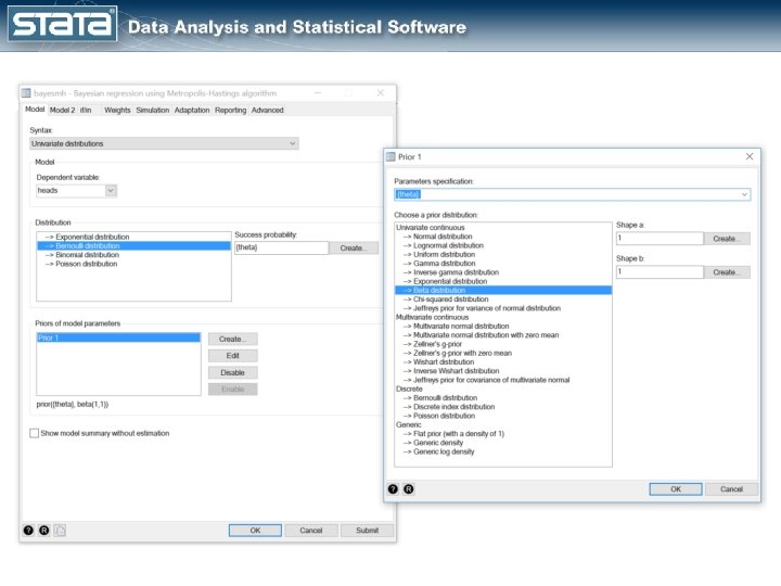
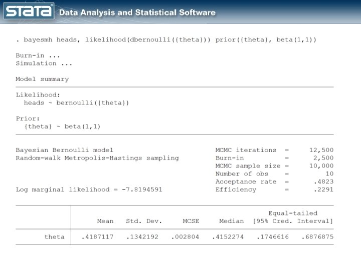
The bayesmh command bayesmh heads, likelihood(dbernoulli({theta})) prior({theta}, beta(1, 1)) ///

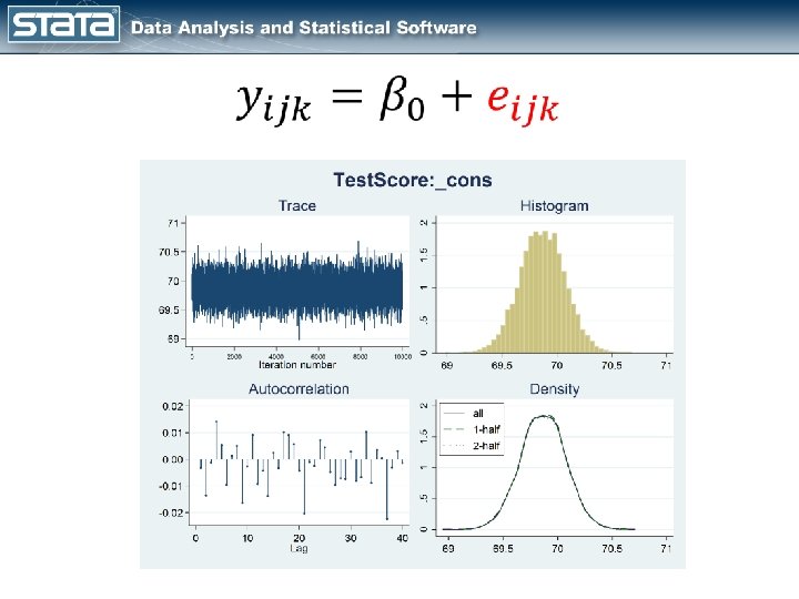
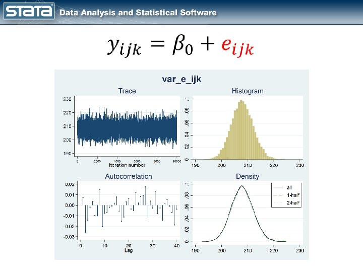
Diagnostic Plots bayesgraph diagnostics {theta}

Outline • • • Introduction to Multilevel Models Introduction to Longitudinal Models Introduction to Bayesian Analysis Bayesian Multilevel Models Bayesian Longitudinal Models
) prior({Test. Score: _cons}, block({Test. Score: _cons}, normal(0,")
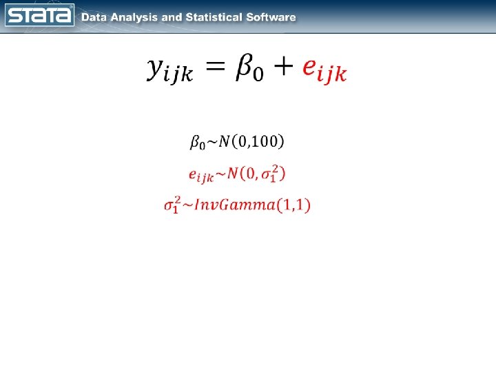
#delimit ; bayesmh Test. Score, likelihood(normal({var_e_ijk})) prior({Test. Score: _cons}, block({Test. Score: _cons}, normal(0, 100)) gibbs) prior({var_e_ijk}, block({var_e_ijk}, igamma(1, 1)) gibbs) burnin(2500) mcmcsize(10000) thinning(1) rseed(14) ; #delimit cr

. bayesstats summary {Test. Score: _cons} {var_e_ijk} Posterior summary statistics MCMC sample size = 10, 000 ---------------------------------------| Equal-tailed | Mean Std. Dev. MCSE Median [95% Cred. Interval] -------+--------------------------------Test. Score | _cons | 69. 8668. 2054122. 002054 69. 86751 69. 46435 70. 27004 -------+--------------------------------var_e_ijk | 207. 8967 4. 178773. 041788 207. 8235 199. 8387 216. 2196 ---------------------------------------

. bayesstats summary {Test. Score: _cons} {var_e_ijk} ---------------------------------------| Equal-tailed | Mean Std. Dev. MCSE Median [95% Cred. Interval] -------+--------------------------------Test. Score | _cons | 69. 8668. 2054122. 002054 69. 86751 69. 46435 70. 27004 -------+--------------------------------var_e_ijk | 207. 8967 4. 178773. 041788 207. 8235 199. 8387 216. 2196 --------------------------------------- . mixed Test. Score ---------------------------------------Test. Score | Coef. Std. Err. z P>|z| [95% Conf. Interval] -------+--------------------------------_cons | 69. 89633. 2059166 339. 44 0. 000 69. 49274 70. 29992 -----------------------------------------------------------------------------Random-effects Parameters | Estimate Std. Err. [95% Conf. Interval] ---------------+------------------------var(Residual) | 207. 768 4. 197548 199. 7017 216. 1601 ---------------------------------------

. bayesstats ess Efficiency summaries MCMC sample size = 10, 000 --------------------------| ESS Corr. time Efficiency -------+-------------------Test. Score | _cons | 10000. 00 1. 0000 -------+-------------------var_e_ijk | 10000. 00 1. 0000 --------------------------
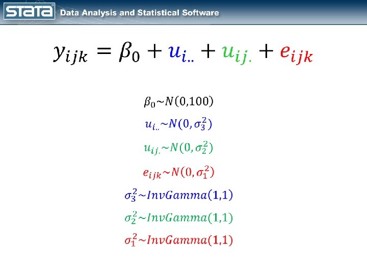

fvset base none classroom fvset base none child #delimit ; bayesmh Test. Score i. classroom#i. child, noconstant likelihood(normal({var_e_ijk})) prior({Test. Score: i. classroom} , normal({Test. Score: _cons}, {var_u_i} )) prior({Test. Score: i. classroom#i. child} , normal(0 , {var_u_0 ij} )) prior({Test. Score: _cons}, normal(0, 100)) prior({var_u_i}, prior({var_u_0 ij}, prior({var_e_ijk}, igamma(1, 1)) block({Test. Score: i. classroom}, block({Test. Score: i. classroom#i. child}, block({Test. Score: _cons}, block({var_e_ijk}, block({var_u_0 ij}, block({var_u_i}, reffects) gibbs) exclude({Test. Score: i. classroom} {Test. Score: i. classroom#i. child} ) burnin(2500) mcmcsize(10000) thinning(1) rseed(14) ; #delimit cr

fvset base none classroom fvset base none child #delimit ; bayesmh Test. Score i. classroom#i. child, noconstant likelihood(normal({var_e_ijk})) prior({Test. Score: _cons}, block({Test. Score: _cons}, normal(0, 100)) gibbs) prior({Test. Score: i. classroom} , prior({var_u_i}, block({Test. Score: i. classroom}, block({var_u_i}, normal({Test. Score: _cons}, igamma(1, 1)) reffects) gibbs) prior({Test. Score: i. classroom#i. child} , prior({var_u_0 ij}, block({Test. Score: i. classroom#i. child}, block({var_u_0 ij}, normal(0 igamma(1, 1)) reffects) gibbs) prior({var_e_ijk}, block({var_e_ijk}, igamma(1, 1)) gibbs) exclude({Test. Score: i. classroom} {Test. Score: i. classroom#i. child} ) burnin(2500) mcmcsize(10000) thinning(1) rseed(14) ; #delimit cr {var_u_i} )) , {var_u_0 ij} ))

. bayesstats summary {Test. Score: _cons} {var_u_i} {var_u_0 ij} {var_e_ijk} Posterior summary statistics MCMC sample size = 10, 000 ---------------------------------------| Equal-tailed | Mean Std. Dev. MCSE Median [95% Cred. Interval] -------+--------------------------------Test. Score | _cons | 69. 72014. 5377208. 024289 69. 73674 68. 62063 70. 76261 -------+--------------------------------var_u_i | 3. 464591 2. 022687. 143491 3. 088572. 7887336 8. 762788 var_u_0 ij | 70. 24564 4. 876976. 130908 70. 00921 61. 17145 80. 22329 var_e_ijk | 134. 2691 2. 953484. 046286 134. 2447 128. 6055 140. 0799 ---------------------------------------
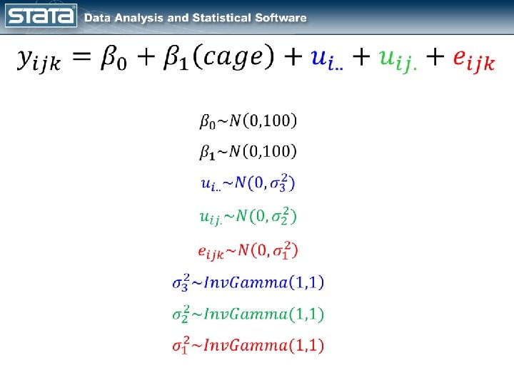

fvset base none classroom fvset base none child #delimit ; bayesmh Test. Score cage i. classroom#i. child, noconstant likelihood(normal({var_e_ijk})) prior({Test. Score: i. classroom}, prior({Test. Score: i. classroom#i. child}, normal({Test. Score: _cons}, {var_u_i} )) normal(0 , {var_u_0 ij})) prior({Test. Score: _cons}, prior({Test. Score: cage}, normal(0, 100)) prior({var_u_i}, prior({var_u_0 ij}, prior({var_e_ijk}, igamma(1, 1)) block({Test. Score: i. classroom}, block({Test. Score: i. classroom#i. child}, block({Test. Score: _cons}, block({Test. Score: cage}, block({var_e_ijk}, block({var_u_0 ij}, block({var_u_i}, reffects) gibbs) gibbs) exclude({Test. Score: i. classroom} {Test. Score: i. classroom#i. child}) burnin(2500) mcmcsize(10000) thinning(1) rseed(14) ; #delimit cr

. bayesstats summary {Test. Score: _cons cage} {var_u_i} {var_u_0 ij} {var_e_ijk} Posterior summary statistics MCMC sample size = 10, 000 ---------------------------------------| Equal-tailed | Mean Std. Dev. MCSE Median [95% Cred. Interval] -------+--------------------------------Test. Score | _cons | 69. 65154. 5437084. 028578 69. 66716 68. 5602 70. 70201 cage | 2. 79475. 0706715. 000707 2. 794595 2. 657682 2. 934435 -------+--------------------------------var_u_i | 3. 631368 2. 000119. 136529 3. 240325. 9996005 8. 539325 var_u_0 ij | 75. 1314 4. 91563. 120718 74. 88609 66. 11253 85. 44937 var_e_ijk | 97. 91347 2. 14513. 035897 97. 88418 93. 78256 102. 1715 ---------------------------------------
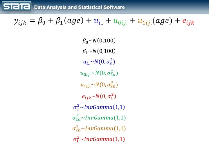

fvset base none classroom fvset base none child #delimit ; bayesmh Test. Score cage i. classroom#i. child#c. cage, noconstant likelihood(normal({var_e_ijk})) prior({Test. Score: i. classroom}, prior({Test. Score: i. classroom#i. child#c. cage}, normal({Test. Score: _cons}, {var_u_i} )) normal(0 , {var_u_0 ij} )) normal(0 , {var_u_1 ij} )) prior({Test. Score: _cons}, prior({Test. Score: cage}, normal(0, 100)) prior({var_u_i}, prior({var_u_0 ij}, prior({var_u_1 ij}, prior({var_e_ijk}, igamma(1, block({Test. Score: i. classroom}, block({Test. Score: i. classroom#i. child#c. cage}, block({Test. Score: _cons}, block({Test. Score: cage}, block({var_e_ijk}, block({var_u_0 ij}, block({var_u_1 ij}, block({var_u_i}, reffects) gibbs) gibbs) 1)) 1)) exclude({Test. Score: i. classroom} {Test. Score: i. classroom#i. child#c. cage}) burnin(2500) mcmcsize(10000) thinning(1) rseed(1234) ; #delimit cr

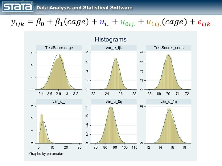
. bayesstats summary {Test. Score: _cons cage} {var_u_i} {var_u_0 ij} {var_u_1 ij} {var_e_ijk} Posterior summary statistics MCMC sample size = 10, 000 ---------------------------------------| Equal-tailed | Mean Std. Dev. MCSE Median [95% Cred. Interval] -------+--------------------------------Test. Score | _cons | 70. 00452. 5359235. 061718 70. 00418 68. 96884 71. 07677 cage | 2. 787785. 1401167. 014216 2. 797113 2. 504285 3. 038121 -------+--------------------------------var_u_i | 3. 554836 2. 183278. 381335 3. 084801. 8301128 9. 103603 var_u_0 ij | 85. 82399 4. 821769. 092891 85. 68783 76. 77357 95. 77512 var_u_1 ij | 15. 57897. 8814715. 011979 15. 54308 13. 95306 17. 40733 var_e_ijk | 25. 27552. 6012595. 013229 25. 26914 24. 11694 26. 47017 ---------------------------------------

. bayesstats summary {Test. Score: _cons cage} {var_u_i} {var_u_0 ij} {var_u_1 ij} {var_e_ijk} ---------------------------------------| Equal-tailed | Mean Std. Dev. MCSE Median [95% Cred. Interval] -------+--------------------------------Test. Score | _cons | 70. 00452. 5359235. 061718 70. 00418 68. 96884 71. 07677 cage | 2. 787785. 1401167. 014216 2. 797113 2. 504285 3. 038121 -------+--------------------------------var_u_i | 3. 554836 2. 183278. 381335 3. 084801. 8301128 9. 103603 var_u_0 ij | 85. 82399 4. 821769. 092891 85. 68783 76. 77357 95. 77512 var_u_1 ij | 15. 57897. 8814715. 011979 15. 54308 13. 95306 17. 40733 var_e_ijk | 25. 27552. 6012595. 013229 25. 26914 24. 11694 26. 47017 --------------------------------------- . mixed Test. Score cage || classroom: || child: cage ---------------------------------------Test. Score | Coef. Std. Err. z P>|z| [95% Conf. Interval] -------+--------------------------------cage | 2. 795204. 1533364 18. 23 0. 000 2. 49467 3. 095738 _cons | 69. 89633. 5487249 127. 38 0. 000 68. 82085 70. 97181 -----------------------------------------------------------------------------Random-effects Parameters | Estimate Std. Err. [95% Conf. Interval] ---------------+------------------------classroom: Identity | var(_cons) | 3. 474859 1. 909333 1. 18366 10. 20111 ---------------+------------------------child: Independent | var(cage) | 15. 55556. 880006 13. 92296 17. 3796 var(_cons) | 85. 53776 4. 835572 76. 5664 95. 5603 ---------------+------------------------var(Residual) | 25. 2807. 6043242 24. 12357 26. 49334 ---------------------------------------

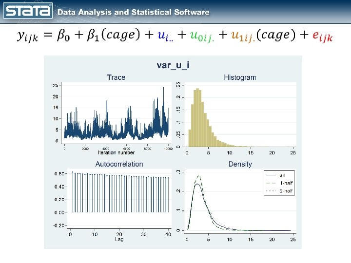
. bayesstats ess Efficiency summaries MCMC sample size = 10, 000 --------------------------| ESS Corr. time Efficiency -------+-------------------Test. Score | cage | 97. 14 102. 94 0. 0097 -------+-------------------var_e_ijk | 2065. 65 4. 84 0. 2066 -------+-------------------Test. Score | _cons | 75. 40 132. 62 0. 0075 -------+-------------------var_u_i | 32. 78 305. 07 0. 0033 var_u_0 ij | 2694. 42 3. 71 0. 2694 var_u_1 ij | 5414. 58 1. 85 0. 5415 --------------------------

. bayesstats ic Linear. Regression Var. Comp Fixed. Slope Rand. Slope, diconly Deviance information criterion --------------| DIC ---------+-----Linear. Regression | 40058. 05 Var. Comp | 38470. 37 Fixed. Slope | 36960. 49 Rand. Slope | 31066. 84 --------------

Further Information • Youtube Videos – Introduction to Bayesian Statistics, part 1: The basic concepts – Introduction to Bayesian Statistics, part 2: MCMC and the Metropolis Hastings algorithm – Item Response Theory Playlist • Blog Entries – Bayesian binary item response theory models using bayesmh – Spotlight on irt

Questions? chuber@stata. com
- Slides: 103