MultilevelLongitudinal Models Using Stata Chuck Huber Ph D

Multilevel/Longitudinal Models Using Stata Chuck Huber, Ph. D Stata. Corp chuber@stata. com University of Michigan – Ann Arbor May 11, 2016

Outline • • The Simulated Dataset Multilevel models for continuous data Fixed vs random effects Multilevel models for binary data Multilevel models for survival data Multilevel structural equation models Bayesian multilevel models
 and")
The Simulated Dataset • This dataset contains repeated measurements of total cholesterol (chol) and systolic blood pressure (sbp) over 7 -8 years. • The patients are nested within three different physician practices. • The final measurement occurred when the patients survived a severe myocardial infarction. • Time-to-death survival data were then collected on these patients.

The Simulated Dataset

The Simulated Dataset

The Simulated Dataset

The Simulated Dataset

The Simulated Dataset

The Simulated Dataset Physician 1 Physician 2 Physician 3

The Simulated Dataset

Outline • • The Simulated Dataset Multilevel models for continuous data Fixed vs random effects Multilevel models for binary data Multilevel models for survival data Multilevel structural equation models Bayesian multilevel models

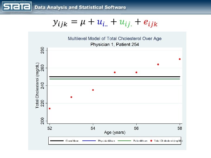
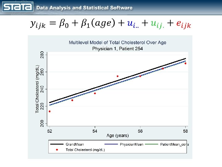
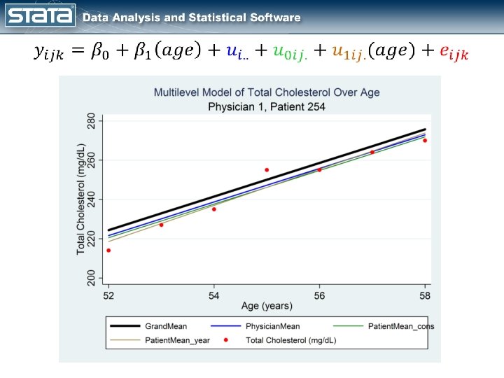
Three Level Models Physician Patient Observations Repeated observations within patients treated by the same physician may be correlated

Observed Fixed Random
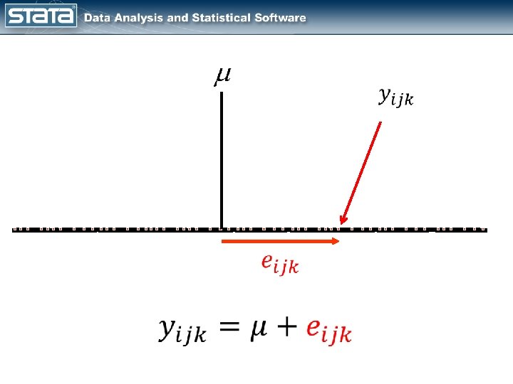

Observed Fixed Random

physician mean patient mean
 cons) n (_ a e m t n e pati")
Systolic Blood Pressure (mm/Hg) cons) n (_ a e m t n e pati dom n a tr e p o l s ien t a p ns) o c _ ( n a n me physicia 30 Age (years) 50

How do we do this in Stata?
 patient mean physician mean grand mean 30 Age (years) 50")
Systolic Blood Pressure (mm/Hg) patient mean physician mean grand mean 30 Age (years) 50

. mixed chol, || physician: || patient: ---------------------------------------chol | Coef. Std. Err. z P>|z| [95% Conf. Interval] -------+--------------------------------_cons | 250. 0533 1. 253489 199. 49 0. 000 247. 5965 252. 5101 -----------------------------------------------------------------------------Random-effects Parameters | Estimate Std. Err. [95% Conf. Interval] ---------------+------------------------physician: Identity | var(_cons) | 4. 228256 3. 849052. 7100652 25. 17818 ---------------+------------------------patient: Identity | var(_cons) | 1. 98 e-19 5. 10 e-19 1. 29 e-21 3. 06 e-17 ---------------+------------------------var(Residual) | 339. 8134 10. 49483 319. 8541 361. 0182 ---------------------------------------LR test vs. linear model: chi 2(2) = 19. 14 Prob > chi 2 = 0. 0001
 ean patient m ean nm physicia 30 Age (years) 50")
Systolic Blood Pressure (mm/Hg) ean patient m ean nm physicia 30 Age (years) 50

. mixed chol cage, || physician: || patient: ---------------------------------------chol | Coef. Std. Err. z P>|z| [95% Conf. Interval] -------+--------------------------------cage | 8. 552381. 0705304 121. 26 0. 000 8. 414144 8. 690618 _cons | 250. 0533 1. 25345 199. 49 0. 000 247. 5966 252. 5101 -----------------------------------------------------------------------------Random-effects Parameters | Estimate Std. Err. [95% Conf. Interval] ---------------+------------------------physician: Identity | var(_cons) | 4. 602921 3. 848604. 8939747 23. 69965 ---------------+------------------------patient: Identity | var(_cons) | 5. 079615. 9282736 3. 550407 7. 267475 ---------------+------------------------var(Residual) | 41. 78608 1. 392869 39. 14337 44. 6072 ---------------------------------------LR test vs. linear model: chi 2(2) = 241. 67 Prob > chi 2 = 0. 0000
 cons) n (_ a e m t n e pati")
Systolic Blood Pressure (mm/Hg) cons) n (_ a e m t n e pati dom n a tr e p o l s ien t a p ns) o c _ ( n a n me physicia 30 Age (years) 50
 ---------------------------------------chol | Coef. Std.")
. mixed chol cage, || physician: || patient: cage, cov(indep) ---------------------------------------chol | Coef. Std. Err. z P>|z| [95% Conf. Interval] -------+--------------------------------cage | 8. 552381. 1242629 68. 82 0. 000 8. 30883 8. 795932 _cons | 250. 0533 1. 253464 199. 49 0. 000 247. 5966 252. 5101 -----------------------------------------------------------------------------Random-effects Parameters | Estimate Std. Err. [95% Conf. Interval] ---------------+------------------------physician: Identity | var(_cons) | 4. 603026 3. 848763. 8939679 23. 70091 ---------------+------------------------patient: Independent | var(cage) | 3. 768022. 3795468 3. 092952 4. 590432 var(_cons) | 7. 59163. 9154443 5. 993659 9. 615636 ---------------+------------------------var(Residual) | 24. 20199. 8837314 22. 53043 25. 99756 ---------------------------------------LR test vs. linear model: chi 2(3) = 721. 05 Prob > chi 2 = 0. 0000
4)) mariginsplot")
margins, at(cage=(-4(1)4)) mariginsplot

Outline • • The Simulated Dataset Multilevel models for continuous data Fixed vs random effects Multilevel models for binary data Multilevel models for survival data Multilevel structural equation models Bayesian multilevel models

Fixed versus Random Effects physician mean patient mean

patient mean

Fixed versus Random Effects Physician treated as a fixed effect Observed Random Fixed Physician treated as a random effect Observed Fixed Random

Physician Treated as a Random Effect. mixed chol cage || physician: || patient: cage , stddev nolog noheader /// ---------------------------------------chol | Coef. Std. Err. z P>|z| [95% Conf. Interval] -------+--------------------------------cage | 8. 552381. 1242629 68. 82 0. 000 8. 30883 8. 795932 _cons | 250. 0533 1. 253464 199. 49 0. 000 247. 5966 252. 5101 -----------------------------------------------------------------------------Random-effects Parameters | Estimate Std. Err. [95% Conf. Interval] ---------------+------------------------physician: Identity | sd(_cons) | 2. 145466. 8969524. 9454987 4. 868358 ---------------+------------------------patient: Independent | sd(cage) | 1. 941139. 0977639 1. 758679 2. 142529 sd(_cons) | 2. 755291. 1661248 2. 448195 3. 100909 ---------------+------------------------sd(Residual) | 4. 919552. 0898183 4. 746623 5. 09878 ---------------------------------------LR test vs. linear model: chi 2(3) = 721. 05 Prob > chi 2 = 0. 0000

Physician Treated as a Fixed Effect. mixed chol cage ibn. physician, nocons || patient: cage , stddev nolog noheader ---------------------------------------chol | Coef. Std. Err. z P>|z| [95% Conf. Interval] -------+--------------------------------cage | 8. 552381. 1242629 68. 82 0. 000 8. 30883 8. 795932 | physician | 1 | 250. 4871. 330735 757. 37 0. 000 249. 8389 251. 1354 2 | 252. 4686. 330735 763. 36 0. 000 251. 8203 253. 1168 3 | 247. 2043. 330735 747. 44 0. 000 246. 5561 247. 8525 -----------------------------------------------------------------------------Random-effects Parameters | Estimate Std. Err. [95% Conf. Interval] ---------------+------------------------patient: Independent | sd(cage) | 1. 941139. 0977639 1. 758679 2. 142529 sd(_cons) | 2. 735167. 1648911 2. 430349 3. 078216 ---------------+------------------------sd(Residual) | 4. 919552. 0898183 4. 746624 5. 098781 ---------------------------------------LR test vs. linear model: chi 2(2) = 533. 65 Prob > chi 2 = 0. 0000 ///

Outline • • The Simulated Dataset Multilevel models for continuous data Fixed vs random effects Multilevel models for binary data Multilevel models for survival data Multilevel structural equation models Bayesian multilevel models

Multilevel Models for GLMs

Multilevel Logistic Regression. melogit Hi. BP cage i. sex || physician: || patient: cage, or nolog Mixed-effects logistic regression Integration method: mvaghermite Number of obs = 2, 100 Integration pts. = 7 Wald chi 2(2) = 66. 75 Log likelihood = -1274. 1098 Prob > chi 2 = 0. 0000 -----------------------------------------Hi. BP | Odds Ratio Std. Err. z P>|z| [95% Conf. Interval] ---------+--------------------------------cage | 1. 498393. 0741657 8. 17 0. 000 1. 359859 1. 65104 | sex | Male |. 9906147. 1350889 -0. 07 0. 945. 7582763 1. 294142 _cons |. 5702334. 0833962 -3. 84 0. 000. 4281195. 7595219 ---------+--------------------------------physician | var(_cons)|. 0347844. 0397053. 0037133. 3258408 ---------+--------------------------------physician>patient | var(cage)|. 3894626. 0728996. 2698596. 5620742 var(_cons)|. 5086553. 1356728. 3015671. 8579525 ------------------------------------------
4)) marginsplot")
Multilevel Logistic Regression margins sex, at(cage=(-4(1)4)) marginsplot

Multilevel Logistic Regression. melogit Hi. BP cage i. sex ibn. physician, nocons || patient: cage, or nolog Integration method: mvaghermite Integration pts. = 7 Wald chi 2(5) = 127. 54 Log likelihood = -1270. 7301 Prob > chi 2 = 0. 0000 ---------------------------------------Hi. BP | Odds Ratio Std. Err. z P>|z| [95% Conf. Interval] -------+--------------------------------cage | 1. 498201. 0741319 8. 17 0. 000 1. 359728 1. 650775 | sex | Male |. 9945755. 1349149 -0. 04 0. 968. 7623803 1. 297489 | physician | 1 |. 7676037. 1029827 -1. 97 0. 049. 5901179. 9984708 2 |. 4559589. 0636761 -5. 62 0. 000. 346779. 599513 3 |. 5271314. 0731874 -4. 61 0. 000. 4015478. 6919912 | _cons | 1 (omitted) -------+--------------------------------patient | var(cage)|. 3891293. 072832. 2696357. 5615786 var(_cons)|. 4948104. 1335798. 2915056. 8399058 ---------------------------------------
4)) marginsplot")
Multilevel Logistic Regression margins sex, at(cage=(-4(1)4)) marginsplot

Outline • • The Simulated Dataset Multilevel models for continuous data Fixed vs random effects Multilevel models for binary data Multilevel models for survival data Multilevel structural equation models Bayesian multilevel models

Multilevel Survival Data Physician 1 Physician 2 Physician 3

Multilevel Survival Data

Multilevel Survival Data

Multilevel Survival Data

Multilevel Survival Data
 at 2(sex=1)")
Multilevel Survival Data stcurve, survival marginal at 1(sex=0) at 2(sex=1)
60)) marginsplot")
Multilevel Survival Data margins sex, at(age_mi=(50(2)60)) marginsplot

Outline • • The Simulated Dataset Multilevel models for continuous data Fixed vs random effects Multilevel models for binary data Multilevel models for survival data Multilevel structural equation models Bayesian multilevel models

Multilevel Structural Equation Models

Multilevel Structural Equation Models
60)) marginsplot")
Multilevel Structural Equation Models margins sex, at(age_mi=(50(2)60)) marginsplot
![Multilevel Structural Equation Models gsem (chol <- cage i. sex M 1[patient] M 2[patient]#c.](http://slidetodoc.com/presentation_image_h2/82092a6e135eb52dbd117e75ee2966e9/image-53.jpg "Multilevel Structural Equation Models gsem (chol <- cage i. sex M 1[patient] M 2[patient]#c.")
Multilevel Structural Equation Models gsem (chol <- cage i. sex M 1[patient] M 2[patient]#c. cage) (sbp <- cage i. sex M 3[patient] M 4[patient]#c. cage), cov(e. sbp*e. chol) covstruct(_lexogenous, diagonal) latent(M 1 M 2 M 3 M 4) /// ///
60)) marginsplot")
Multilevel Structural Equation Models margins sex, at(age_mi=(50(2)60)) marginsplot
![Multilevel Structural Equation Models gsem (time <- age chol Hi. BP M 2[physician], family(exponential,](http://slidetodoc.com/presentation_image_h2/82092a6e135eb52dbd117e75ee2966e9/image-55.jpg "Multilevel Structural Equation Models gsem (time <- age chol Hi. BP M 2[physician], family(exponential,")
Multilevel Structural Equation Models gsem (time <- age chol Hi. BP M 2[physician], family(exponential, failure(dead) ph) link(log )) /// (Hi. BP <- age M 1[physician], family(bernoulli) link(logit)) /// (chol <- age M 3[physician]) /// , covstruct(_lexogenous, diagonal) /// latent(M 1 M 2 M 3) nolog

Multilevel Structural Equation Models

Multilevel Structural Equation Models

Outline • • The Simulated Dataset Multilevel models for continuous data Fixed vs random effects Multilevel models for binary data Multilevel models for survival data Multilevel structural equation models Bayesian multilevel models
) noconstant prior({chol: i. patient}, normal({chol:")
Bayesian Multilevel Models bayesmh chol i. patient#c. cage, likelihood(normal({var_0})) noconstant prior({chol: i. patient}, normal({chol: _cons}, {var_patient})) prior({chol: i. patient#c. cage}, normal({chol: cage}, {var_cage})) prior({chol: _cons}, normal(0, 100)) prior({chol: cage}, normal(0, 100)) prior({var_0}, igamma(0. 001, 0. 001)) prior({var_patient}, igamma(0. 001, 0. 001)) prior({var_cage}, igamma(0. 001, 0. 001)) block({var_0}, gibbs) block({var_patient}, gibbs) block({var_cage}, gibbs) block({chol: i. patient#c. cage}, gibbs) block({chol: _cons}, gibbs) burnin(5000) mcmcsize(10000) thinning(1) rseed(14) dots notable

Bayesian Multilevel Models

Bayesian Multilevel Models

Outline • • The Simulated Dataset Multilevel models for continuous data Fixed vs random effects Multilevel models for binary data Multilevel models for survival data Multilevel structural equation models Bayesian multilevel models

For more information • Videos – Introduction to Multilevel Models Part 1 – Introduction to Multilevel Models Part 2 • Blogs – Introduction to Multilevel Models Part 1 – Introduction to Multilevel Models Part 2 – How to simulate multilevel/longitudinal data

Questions? chuber@stata. com
- Slides: 64