Artificial Intelligence Neural Networks Copyright 2010 Dieter Fensel

Artificial Intelligence Neural Networks © Copyright 2010 Dieter Fensel and Reto Krummenacher 1

Where are we? # Title 1 Introduction 2 Propositional Logic 3 Predicate Logic 4 Reasoning 5 Search Methods 6 Common. KADS 7 Problem-Solving Methods 8 Planning 9 Software Agents 10 Rule Learning 11 Inductive Logic Programming 12 Formal Concept Analysis 13 Neural Networks 14 Semantic Web and Services 2

Agenda • Motivation • Technical Solution – – – (Artificial) Neural Networks Perceptron Artificial Neural Network Structures Learning and Generalization Expressiveness of Multi-Layer Perceptrons • Illustration by Larger Examples • Summary 3

MOTIVATION 4 4

Motivation • A main motivation behind neural networks is the fact that symbolic rules do not reflect reasoning processes performed by humans. • Biological neural systems can capture highly parallel computations based on representations that are distributed over many neurons. • They learn and generalize from training data; no need for programming it all. . . • They are very noise tolerant – better resistance than symbolic systems. 5

Motivation • Neural networks are stong in: – Learning from a set of examples – Optimizing solutions via constraints and cost functions – Classification: grouping elements in classes – Speech recognition, pattern matching – Non-parametric statistical analysis and regressions 6

TECHNICAL SOLUTIONS 7 7

(Artificial) Neural Networks 8 8

What are Neural Networks? • A biological neural network is composed of groups of chemically connected or functionally associated neurons. • A single neuron may be connected to many other neurons and the total number of neurons and connections in a network may be extensive. • Neurons are highly specialized cells that transmit impulses within animals to cause a change in a target cell such as a muscle effector cell or a glandular cell. • Impulses are noisy “spike trains” of electronical potential. • Apart from the electrical signaling, neurotransmitter diffusion (endogenous chemicals) can effectuate the impulses. 9

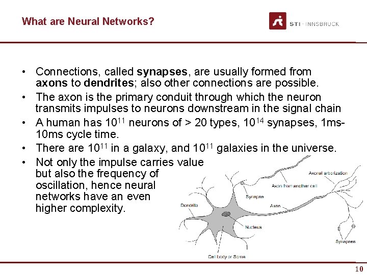
What are Neural Networks? • Connections, called synapses, are usually formed from axons to dendrites; also other connections are possible. • The axon is the primary conduit through which the neuron transmits impulses to neurons downstream in the signal chain • A human has 1011 neurons of > 20 types, 1014 synapses, 1 ms 10 ms cycle time. • There are 1011 in a galaxy, and 1011 galaxies in the universe. • Not only the impulse carries value but also the frequency of oscillation, hence neural networks have an even higher complexity. 10

What are Neural Networks? • Metaphorically speaking, a thought is a specific self-oscillation of a network of neurons. • The topology of the network determines its resonance. • However, it is the resonance in the brain's interaction with the environment and with itself that creates, reinforces or decouples interaction patterns. • The brain is not a static device, but a device that is created through usage… 11

What are Neural Networks? • What we refer to as Neural Networks, in this course, are mostly Artificial Neural Networks (ANN). • ANN are approximations of biological neural networks and are built of physical devices, or simulated on computers. • ANN are parallel computational entities that consist of multiple simple processing units that are connected in specific ways in order to perform the desired tasks. • Remember: ANN are computationally primitive approximations of the real biological brains. 12

Perceptron 13 13

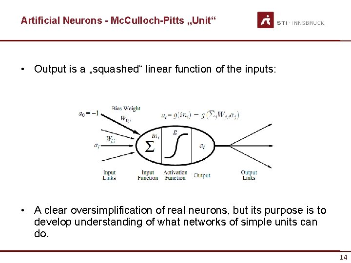
Artificial Neurons - Mc. Culloch-Pitts „Unit“ • Output is a „squashed“ linear function of the inputs: • A clear oversimplification of real neurons, but its purpose is to develop understanding of what networks of simple units can do. 14

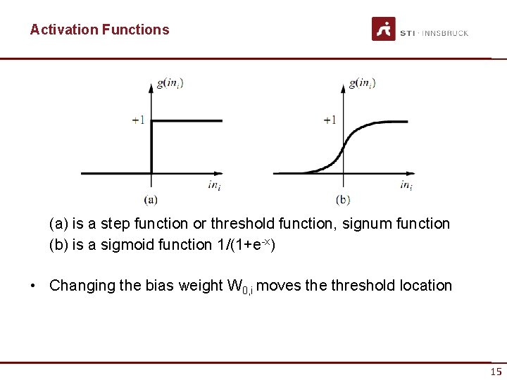
Activation Functions (a) is a step function or threshold function, signum function (b) is a sigmoid function 1/(1+e-x) • Changing the bias weight W 0, i moves the threshold location 15

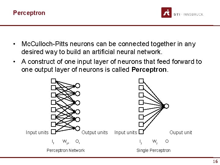
Perceptron • Mc. Culloch-Pitts neurons can be connected together in any desired way to build an artificial neural network. • A construct of one input layer of neurons that feed forward to one output layer of neurons is called Perceptron. Input units Output units Ij Wj, i Oi Perceptron Network Input units Ouput unit Ij Wj O Single Perceptron 16

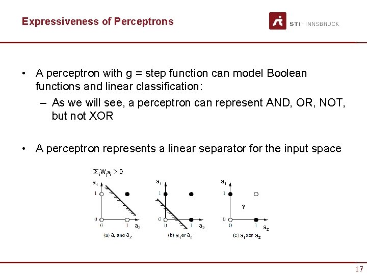
Expressiveness of Perceptrons • A perceptron with g = step function can model Boolean functions and linear classification: – As we will see, a perceptron can represent AND, OR, NOT, but not XOR • A perceptron represents a linear separator for the input space ∑j. Wjaj > 0 a 1 a 1 a 2 a 2 a 1 a 2 17

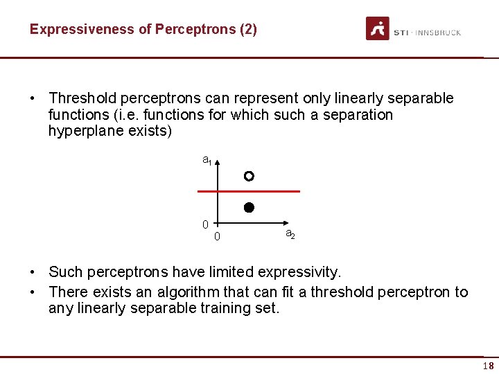
Expressiveness of Perceptrons (2) • Threshold perceptrons can represent only linearly separable functions (i. e. functions for which such a separation hyperplane exists) a 1 0 0 a 2 • Such perceptrons have limited expressivity. • There exists an algorithm that can fit a threshold perceptron to any linearly separable training set. 18

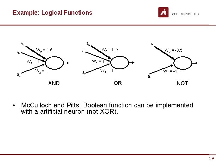
Example: Logical Functions a 0 a 1 W 0 = 1. 5 a 1 W 0 = 0. 5 W 0 = -0. 5 W 1 = 1 a 2 a 0 W 2 = 1 a 2 AND W 2 = 1 a 1 OR W 1 = -1 NOT • Mc. Culloch and Pitts: Boolean function can be implemented with a artificial neuron (not XOR). 19

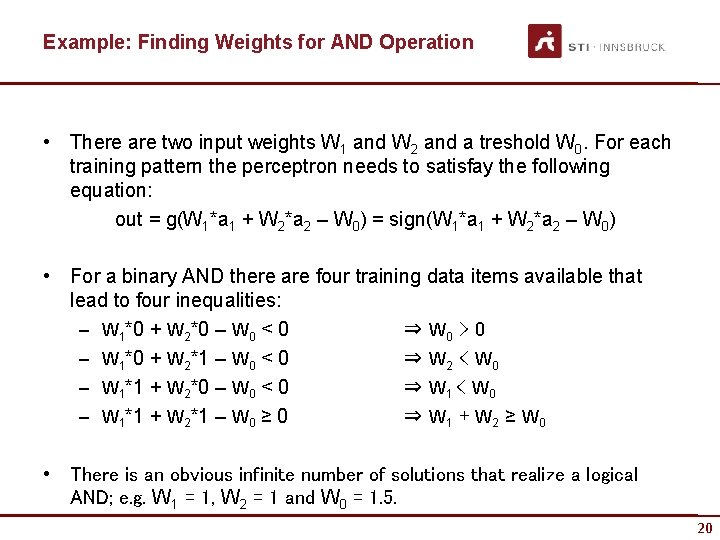
Example: Finding Weights for AND Operation • There are two input weights W 1 and W 2 and a treshold W 0. For each training pattern the perceptron needs to satisfay the following equation: out = g(W 1*a 1 + W 2*a 2 – W 0) = sign(W 1*a 1 + W 2*a 2 – W 0) • For a binary AND there are four training data items available that lead to four inequalities: – W 1*0 + W 2*0 – W 0 < 0 ⇒ W 0 > 0 – W 1*0 + W 2*1 – W 0 < 0 ⇒ W 2 < W 0 – W 1*1 + W 2*0 – W 0 < 0 ⇒ W 1 < W 0 – W 1*1 + W 2*1 – W 0 ≥ 0 ⇒ W 1 + W 2 ≥ W 0 • There is an obvious infinite number of solutions that realize a logical AND; e. g. W 1 = 1, W 2 = 1 and W 0 = 1. 5. 20

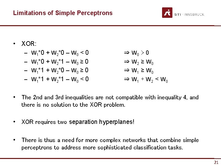
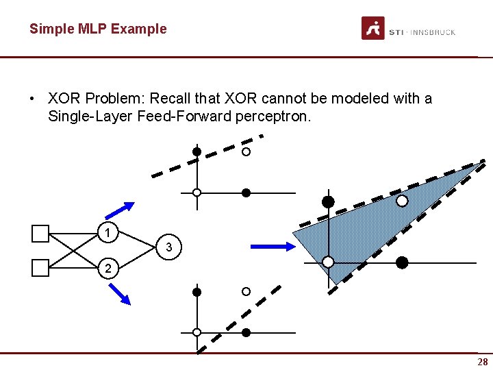
Limitations of Simple Perceptrons • XOR: – W 1*0 + W 2*0 – W 0 < 0 – W 1*0 + W 2*1 – W 0 ≥ 0 – W 1*1 + W 2*0 – W 0 ≥ 0 – W 1*1 + W 2*1 – W 0 < 0 ⇒ ⇒ W 0 > 0 W 2 ≥ W 0 W 1 + W 2 < W 0 • The 2 nd and 3 rd inequalities are not compatible with inequality 4, and there is no solution to the XOR problem. • XOR requires two separation hyperplanes! • There is thus a need for more complex networks that combine simple perceptrons to address more sophisticated classification tasks. 21

Artificial Neural Network Structures 22 22

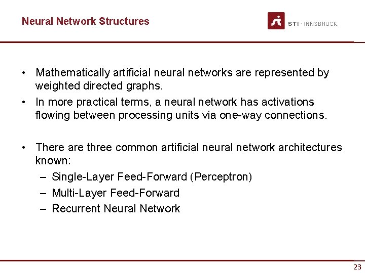
Neural Network Structures • Mathematically artificial neural networks are represented by weighted directed graphs. • In more practical terms, a neural network has activations flowing between processing units via one-way connections. • There are three common artificial neural network architectures known: – Single-Layer Feed-Forward (Perceptron) – Multi-Layer Feed-Forward – Recurrent Neural Network 23

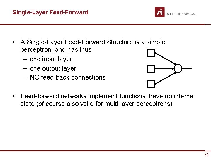
Single-Layer Feed-Forward • A Single-Layer Feed-Forward Structure is a simple perceptron, and has thus – one input layer – one output layer – NO feed-back connections • Feed-forward networks implement functions, have no internal state (of course also valid for multi-layer perceptrons). 24

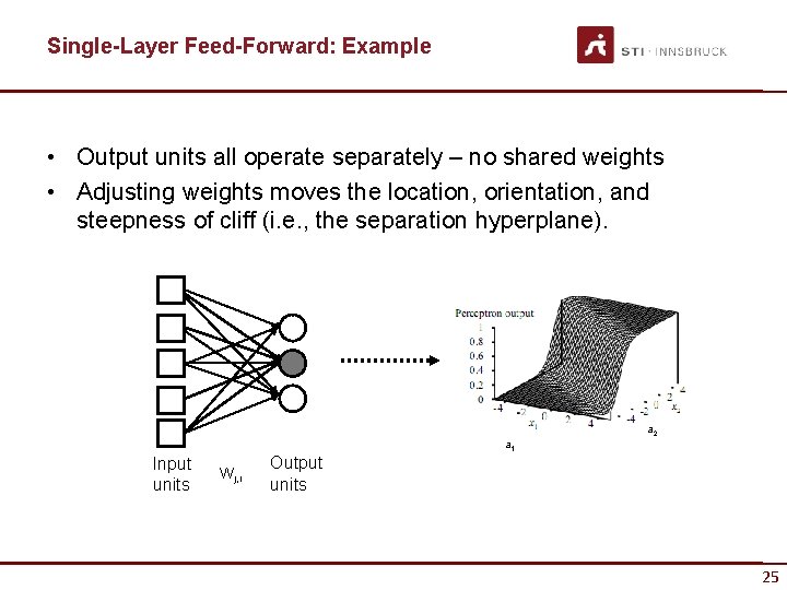
Single-Layer Feed-Forward: Example • Output units all operate separately – no shared weights • Adjusting weights moves the location, orientation, and steepness of cliff (i. e. , the separation hyperplane). a 2 a 1 Input units Wj, i Output units 25

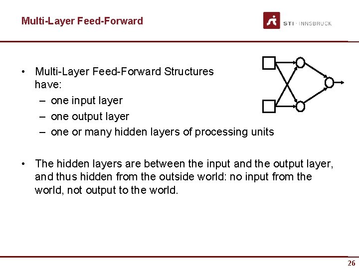
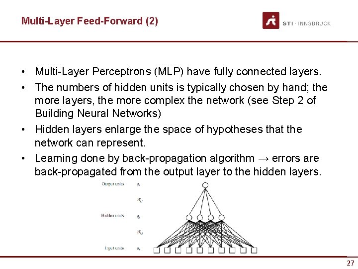
Multi-Layer Feed-Forward • Multi-Layer Feed-Forward Structures have: – one input layer – one output layer – one or many hidden layers of processing units • The hidden layers are between the input and the output layer, and thus hidden from the outside world: no input from the world, not output to the world. 26

Multi-Layer Feed-Forward (2) • Multi-Layer Perceptrons (MLP) have fully connected layers. • The numbers of hidden units is typically chosen by hand; the more layers, the more complex the network (see Step 2 of Building Neural Networks) • Hidden layers enlarge the space of hypotheses that the network can represent. • Learning done by back-propagation algorithm → errors are back-propagated from the output layer to the hidden layers. 27

Simple MLP Example • XOR Problem: Recall that XOR cannot be modeled with a Single-Layer Feed-Forward perceptron. 1 3 2 28

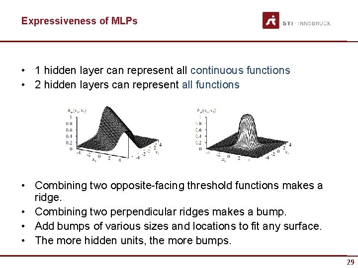
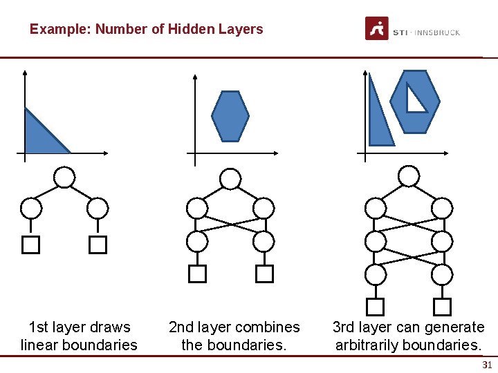
Expressiveness of MLPs • 1 hidden layer can represent all continuous functions • 2 hidden layers can represent all functions • Combining two opposite-facing threshold functions makes a ridge. • Combining two perpendicular ridges makes a bump. • Add bumps of various sizes and locations to fit any surface. • The more hidden units, the more bumps. 29

Number of Hidden Layers • Rule of Thumb 1 Even if the function to learn is slightly non-linear, the generalization may be better with a simple linear model than with a complicated non-linear model; if there is too little data or too much noise to estimate the non-linearities accurately. • Rule of Thumb 2 If there is only one input, there seems to be no advantage to using more than one hidden layer; things get much more complicated when there are two or more inputs. 30

Example: Number of Hidden Layers 1 st layer draws linear boundaries 2 nd layer combines the boundaries. 3 rd layer can generate arbitrarily boundaries. 31

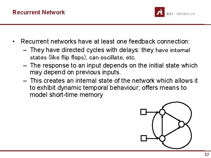
Recurrent Network • Recurrent networks have at least one feedback connection: – They have directed cycles with delays: they have internal states (like flip flops), can oscillate, etc. – The response to an input depends on the initial state which may depend on previous inputs. – This creates an internal state of the network which allows it to exhibit dynamic temporal behaviour; offers means to model short-time memory 32

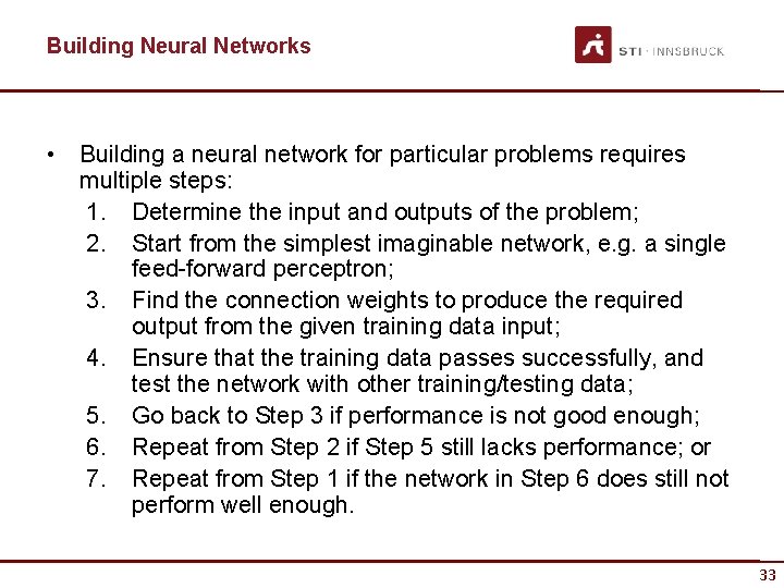
Building Neural Networks • Building a neural network for particular problems requires multiple steps: 1. Determine the input and outputs of the problem; 2. Start from the simplest imaginable network, e. g. a single feed-forward perceptron; 3. Find the connection weights to produce the required output from the given training data input; 4. Ensure that the training data passes successfully, and test the network with other training/testing data; 5. Go back to Step 3 if performance is not good enough; 6. Repeat from Step 2 if Step 5 still lacks performance; or 7. Repeat from Step 1 if the network in Step 6 does still not perform well enough. 33

Learning and Generalization 34 34

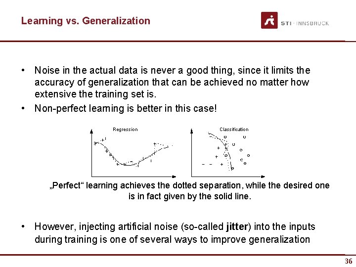
Learning and Generalization • Neural networks have two important aspects to fulfill: – They must learn decision surfaces from training data, so that training data (and test data) are classified correctly; – They must be able to generalize based on the learning process, in order to classify data sets it has never seen before. • Note that there is an important trade-off between the learning behavior and the generalization of a neural network (called overfitting) • The better a network learns to successfully classify a training sequence (that might contain errors) the less flexible it is with respect to arbitrary data. 35

Learning vs. Generalization • Noise in the actual data is never a good thing, since it limits the accuracy of generalization that can be achieved no matter how extensive the training set is. • Non-perfect learning is better in this case! Regression Classification „Perfect“ learning achieves the dotted separation, while the desired one is in fact given by the solid line. • However, injecting artificial noise (so-called jitter) into the inputs during training is one of several ways to improve generalization 36

Estimation of Generalization Error • There are many methods for estimating generalization errors. • Single-sample statistics – Statistical theory provides estimators for the generalization error in non-linear models with a "large" training set. • Split-sample or hold-out validation. – The most commonly used method: reserve some data as a "test set”, which must not be used during training. – The test set must represent the cases that the ANN should generalize to. – A re-run with the random test set provides an unbiased estimate of the generalization error. – The disadvantage of split-sample validation is that it reduces the amount of data available for both training and validation. 37

Estimation of Generalization Error • Cross-validation (e. g. , leave one out). – In k-fold cross-validation the data is divided into k subsets, and the network is trained k times, each time leaving one subset out for computing the error. – The “crossing” makes this method an improvement over splitsampling; it allows all data to be used for training. – The disadvantage of cross-validation is that the network must be re-trained many times (k times in k-fold crossing). • Bootstrapping. – Bootstrapping works on random sub-samples (random shares) that are chosen from the full data set. – Any data item may be selected any number of times for validation. – The sub-samples are repeatedly analyzed. • No matter which method is applied, the estimate of the generalization error of the best network will be optimistic. 38

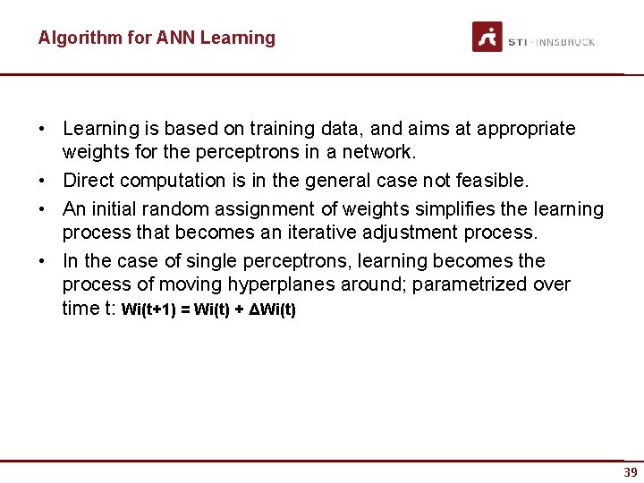
Algorithm for ANN Learning • Learning is based on training data, and aims at appropriate weights for the perceptrons in a network. • Direct computation is in the general case not feasible. • An initial random assignment of weights simplifies the learning process that becomes an iterative adjustment process. • In the case of single perceptrons, learning becomes the process of moving hyperplanes around; parametrized over time t: Wi(t+1) = Wi(t) + ΔWi(t) 39

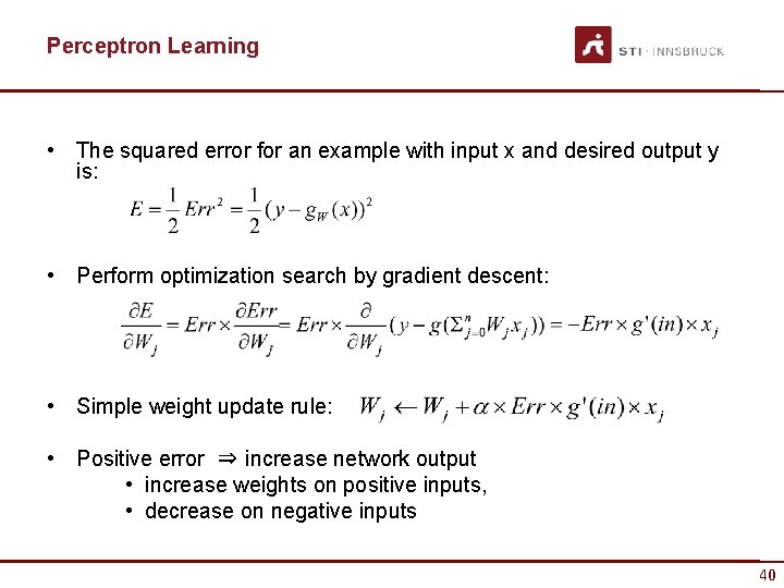
Perceptron Learning • The squared error for an example with input x and desired output y is: • Perform optimization search by gradient descent: • Simple weight update rule: • Positive error ⇒ increase network output • increase weights on positive inputs, • decrease on negative inputs 40

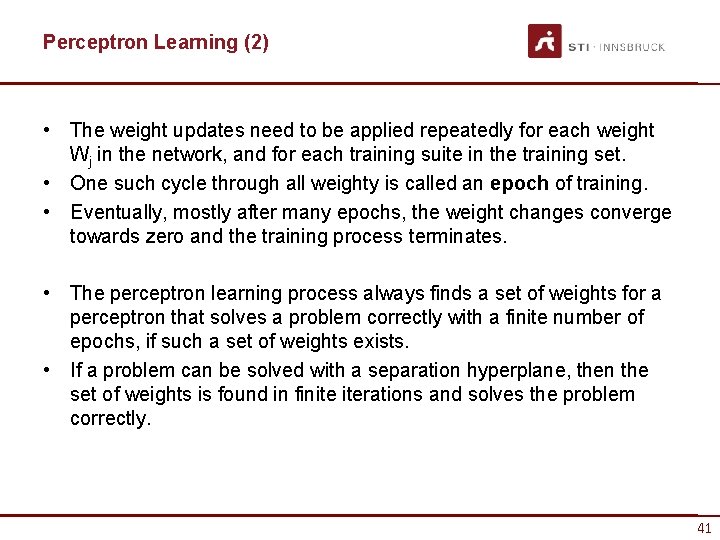
Perceptron Learning (2) • The weight updates need to be applied repeatedly for each weight Wj in the network, and for each training suite in the training set. • One such cycle through all weighty is called an epoch of training. • Eventually, mostly after many epochs, the weight changes converge towards zero and the training process terminates. • The perceptron learning process always finds a set of weights for a perceptron that solves a problem correctly with a finite number of epochs, if such a set of weights exists. • If a problem can be solved with a separation hyperplane, then the set of weights is found in finite iterations and solves the problem correctly. 41

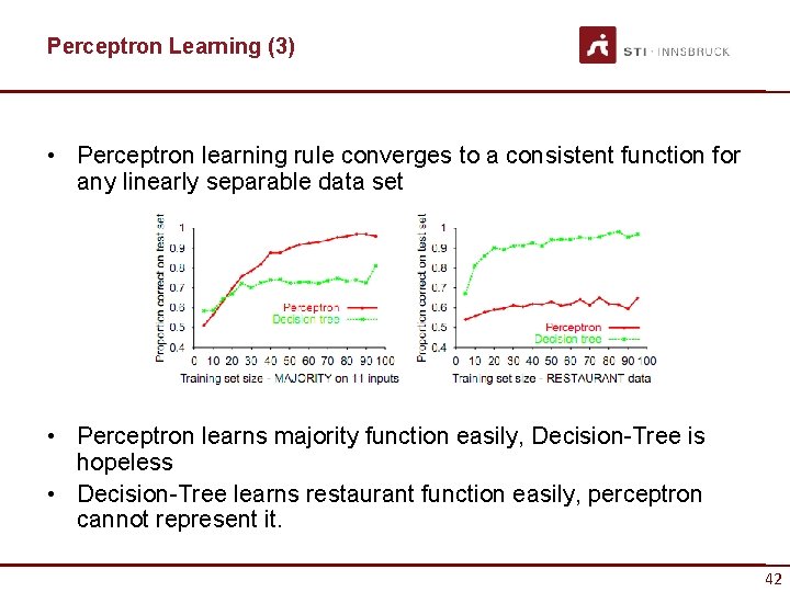
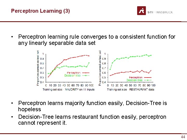
Perceptron Learning (3) • Perceptron learning rule converges to a consistent function for any linearly separable data set • Perceptron learns majority function easily, Decision-Tree is hopeless • Decision-Tree learns restaurant function easily, perceptron cannot represent it. 42

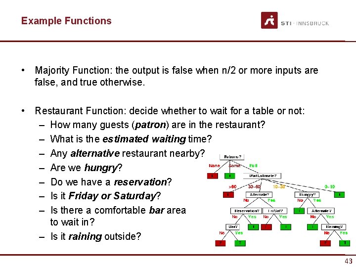
Example Functions • Majority Function: the output is false when n/2 or more inputs are false, and true otherwise. • Restaurant Function: decide whether to wait for a table or not: – How many guests (patron) are in the restaurant? – What is the estimated waiting time? – Any alternative restaurant nearby? – Are we hungry? – Do we have a reservation? – Is it Friday or Saturday? – Is there a comfortable bar area to wait in? – Is it raining outside? 43

Perceptron Learning (3) • Perceptron learning rule converges to a consistent function for any linearly separable data set • Perceptron learns majority function easily, Decision-Tree is hopeless • Decision-Tree learns restaurant function easily, perceptron cannot represent it. 44

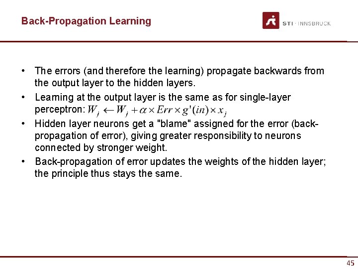
Back-Propagation Learning • The errors (and therefore the learning) propagate backwards from the output layer to the hidden layers. • Learning at the output layer is the same as for single-layer perceptron: • Hidden layer neurons get a "blame" assigned for the error (backpropagation of error), giving greater responsibility to neurons connected by stronger weight. • Back-propagation of error updates the weights of the hidden layer; the principle thus stays the same. 45

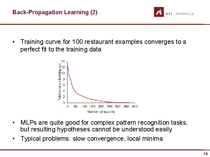
Back-Propagation Learning (2) • Training curve for 100 restaurant examples converges to a perfect fit to the training data • MLPs are quite good for complex pattern recognition tasks, but resulting hypotheses cannot be understood easily • Typical problems: slow convergence, local minima 46

ILLUSTRATION BY AN EXAMPLE 47 47

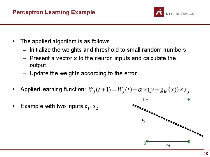
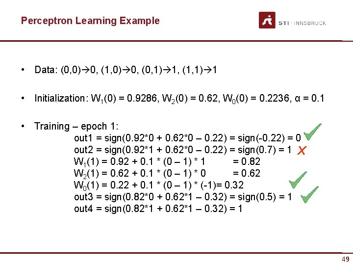
Perceptron Learning Example • The applied algorithm is as follows – Initialize the weights and threshold to small random numbers. – Present a vector x to the neuron inputs and calculate the output. – Update the weights according to the error. • Applied learning function: + 1+ • Example with two inputs x 1, x 2 o 0 x 1 o 1 48

Perceptron Learning Example • Data: (0, 0) 0, (1, 0) 0, (0, 1) 1, (1, 1) 1 • Initialization: W 1(0) = 0. 9286, W 2(0) = 0. 62, W 0(0) = 0. 2236, α = 0. 1 • Training – epoch 1: out 1 = sign(0. 92*0 + 0. 62*0 – 0. 22) = sign(-0. 22) = 0 out 2 = sign(0. 92*1 + 0. 62*0 – 0. 22) = sign(0. 7) = 1 X W 1(1) = 0. 92 + 0. 1 * (0 – 1) * 1 = 0. 82 W 2(1) = 0. 62 + 0. 1 * (0 – 1) * 0 = 0. 62 W 0(1) = 0. 22 + 0. 1 * (0 – 1) * (-1)= 0. 32 out 3 = sign(0. 82*0 + 0. 62*1 – 0. 32) = sign(0. 5) = 1 out 4 = sign(0. 82*1 + 0. 62*1 – 0. 32) = 1 49

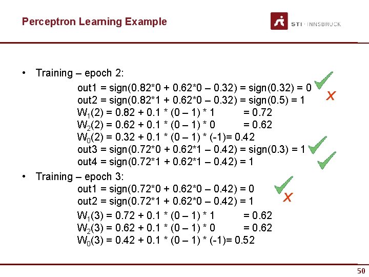
Perceptron Learning Example • Training – epoch 2: out 1 = sign(0. 82*0 + 0. 62*0 – 0. 32) = sign(0. 32) = 0 out 2 = sign(0. 82*1 + 0. 62*0 – 0. 32) = sign(0. 5) = 1 W 1(2) = 0. 82 + 0. 1 * (0 – 1) * 1 = 0. 72 W 2(2) = 0. 62 + 0. 1 * (0 – 1) * 0 = 0. 62 W 0(2) = 0. 32 + 0. 1 * (0 – 1) * (-1)= 0. 42 out 3 = sign(0. 72*0 + 0. 62*1 – 0. 42) = sign(0. 3) = 1 out 4 = sign(0. 72*1 + 0. 62*1 – 0. 42) = 1 • Training – epoch 3: out 1 = sign(0. 72*0 + 0. 62*0 – 0. 42) = 0 X out 2 = sign(0. 72*1 + 0. 62*0 – 0. 42) = 1 W 1(3) = 0. 72 + 0. 1 * (0 – 1) * 1 = 0. 62 W 2(3) = 0. 62 + 0. 1 * (0 – 1) * 0 = 0. 62 W 0(3) = 0. 42 + 0. 1 * (0 – 1) * (-1)= 0. 52 X 50

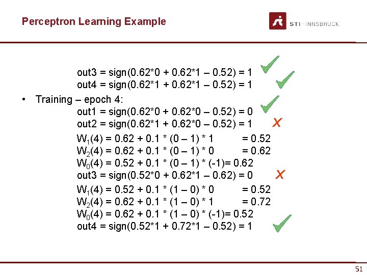
Perceptron Learning Example out 3 = sign(0. 62*0 + 0. 62*1 – 0. 52) = 1 out 4 = sign(0. 62*1 + 0. 62*1 – 0. 52) = 1 • Training – epoch 4: out 1 = sign(0. 62*0 + 0. 62*0 – 0. 52) = 0 X out 2 = sign(0. 62*1 + 0. 62*0 – 0. 52) = 1 W 1(4) = 0. 62 + 0. 1 * (0 – 1) * 1 = 0. 52 W 2(4) = 0. 62 + 0. 1 * (0 – 1) * 0 = 0. 62 W 0(4) = 0. 52 + 0. 1 * (0 – 1) * (-1)= 0. 62 out 3 = sign(0. 52*0 + 0. 62*1 – 0. 62) = 0 X W 1(4) = 0. 52 + 0. 1 * (1 – 0) * 0 = 0. 52 W 2(4) = 0. 62 + 0. 1 * (1 – 0) * 1 = 0. 72 W 0(4) = 0. 62 + 0. 1 * (1 – 0) * (-1)= 0. 52 out 4 = sign(0. 52*1 + 0. 72*1 – 0. 52) = 1 51

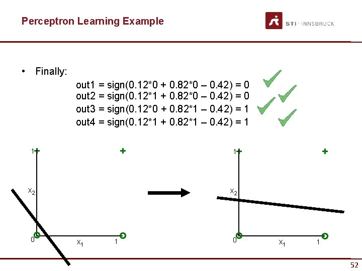
Perceptron Learning Example • Finally: out 1 = sign(0. 12*0 + 0. 82*0 – 0. 42) = 0 out 2 = sign(0. 12*1 + 0. 82*0 – 0. 42) = 0 out 3 = sign(0. 12*0 + 0. 82*1 – 0. 42) = 1 out 4 = sign(0. 12*1 + 0. 82*1 – 0. 42) = 1 + + 1 x 2 o 0 + + 1 x 2 x 1 1 o o 0 x 1 1 o 52

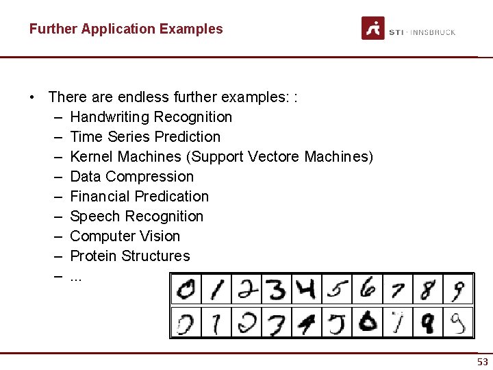
Further Application Examples • There are endless further examples: : – Handwriting Recognition – Time Series Prediction – Kernel Machines (Support Vectore Machines) – Data Compression – Financial Predication – Speech Recognition – Computer Vision – Protein Structures –. . . 53

SUMMARY 54 54

Summary • Most brains have lots of neurons, each neuron approximates a linear-threshold unit. • Perceptrons (one-layer networks) approximate neurons, but are as such insufficiently expressive. • Multi-layer networks are sufficiently expressive; can be trained to deal with generalized data sets, i. e. via error backpropagation. • Multi-layer networks allow for the modeling of arbitrary separation boundaries, while single-layer perceptrons only provide linear boundaries. • Endless number of applications: Handwriting Recognition, Time Series Prediction, Bioinformatics, Kernel Machines (Support Vectore Machines), Data Compression, Financial Predication, Speech Recognition, Computer Vision, Protein Structures. . . 55

REFERENCES 56 56

References Mandatory Readings: • Mc. Culloch, W. S. & Pitts, W. (1943): A Logical Calculus of the Ideas Immanent in Nervous Activity. Bulletin of Mathematical Biophysics 5, pp. 115 -133. • Rosenblatt, F. (1958): The perceptron: a probabilistic model for information storage and organization in the brain. Psychological Reviews 65, pp. 386408. Further Readings: • Elman, J. L. (1990): Finding structure in time. Cognitive Science 14, pp. 179– 211. • Gallant, S. I. (1990): Perceptron-based learning algorithms. IEEE Transactions on Neural Networks 1 (2), pp. 179 -191. • Rumelhart, D. E. , Hinton, G. E. & Williams, R. J. (1986): Learning representations by back-propagating errors. Nature 323, pp. 533 -536. • Supervised learning demo (perceptron learning rule) at http: //lcn. epfl. ch/tutorial/english/perceptron/html/ 57

References Wikipedia References: • http: //en. wikipedia. org/wiki/Biological_neural_networks • http: //en. wikipedia. org/wiki/Artificial_neural_network • http: //en. wikipedia. org/wiki/Perceptron • http: //en. wikipedia. org/wiki/Feedforward_neural_network • http: //en. wikipedia. org/wiki/Recurrent_neural_networks • http: //en. wikipedia. org/wiki/Back_propagation 58

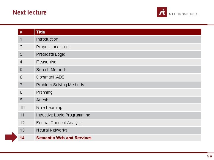
Next lecture # Title 1 Introduction 2 Propositional Logic 3 Predicate Logic 4 Reasoning 5 Search Methods 6 Common. KADS 7 Problem-Solving Methods 8 Planning 9 Agents 10 Rule Learning 11 Inductive Logic Programming 12 Formal Concept Analysis 13 Neural Networks 14 Semantic Web and Services 59

Questions? 60 60