Advanced Topics in Regression Suppression Mediation Analysis Psy

Advanced Topics in Regression: Suppression & Mediation Analysis Psy 252 1

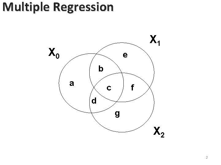
Multiple Regression X 1 X 0 e b a c f d g X 2 2

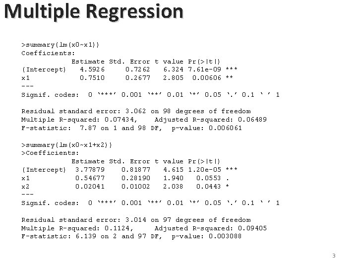
Multiple Regression >summary(lm(x 0~x 1)) Coefficients: Estimate Std. Error t value Pr(>|t|) (Intercept) 4. 5926 0. 7262 6. 324 7. 61 e-09 *** x 1 0. 7510 0. 2677 2. 805 0. 00606 ** --Signif. codes: 0 ‘***’ 0. 001 ‘**’ 0. 01 ‘*’ 0. 05 ‘. ’ 0. 1 ‘ ’ 1 Residual standard error: 3. 062 on 98 degrees of freedom Multiple R-squared: 0. 07434, Adjusted R-squared: 0. 06489 F-statistic: 7. 87 on 1 and 98 DF, p-value: 0. 006061 >summary(lm(x 0~x 1+x 2)) >Coefficients: Estimate Std. Error t value Pr(>|t|) (Intercept) 3. 77879 0. 81877 4. 615 1. 20 e-05 *** x 1 0. 54677 0. 28190 1. 940 0. 0553. x 2 0. 02041 0. 01002 2. 038 0. 0443 * --Signif. codes: 0 ‘***’ 0. 001 ‘**’ 0. 01 ‘*’ 0. 05 ‘. ’ 0. 1 ‘ ’ 1 Residual standard error: 3. 014 on 97 degrees of freedom Multiple R-squared: 0. 1124, Adjusted R-squared: 0. 09405 F-statistic: 6. 139 on 2 and 97 DF, p-value: 0. 003088 3

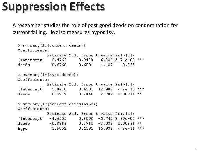
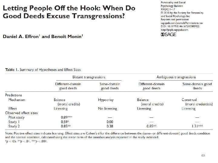
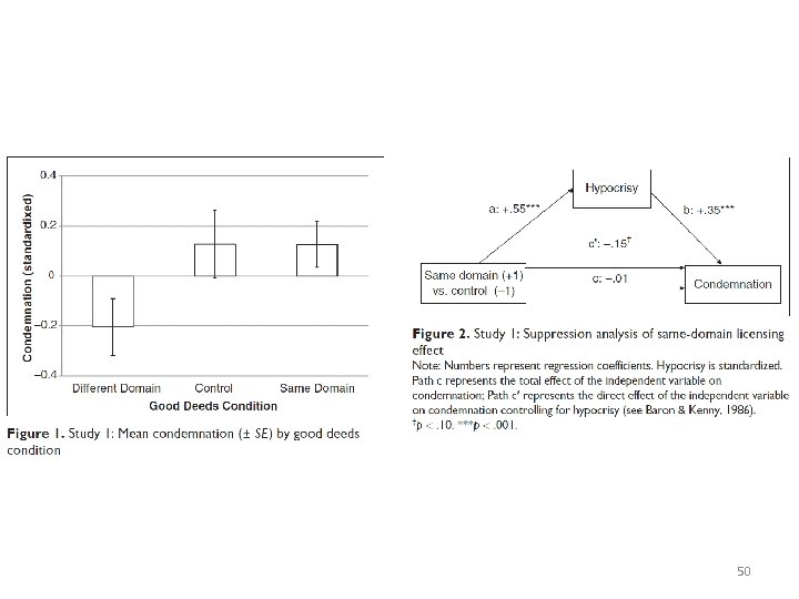
Suppression Effects A researcher studies the role of past good deeds on condemnation for current failing. He also measures hypocrisy. > summary(lm(condemn~deeds)) Coefficients: Estimate Std. Error t value Pr(>|t|) (Intercept) 6. 4764 0. 9488 6. 826 5. 74 e-09 *** deeds 0. 6760 0. 6001 1. 127 0. 265 > summary(lm(hypo~deeds)) Coefficients: Estimate Std. Error t value Pr(>|t|) (Intercept) 5. 8430 0. 4501 12. 982 < 2 e-16 *** deeds 0. 7939 0. 2846 2. 789 0. 00714 ** > summary(lm(condemn~deeds+hypo)) Coefficients: Estimate Std. Error t value Pr(>|t|) (Intercept) -4. 6555 0. 8098 -5. 749 3. 69 e-07 *** deeds -0. 8366 0. 2760 -3. 032 0. 00366 ** hypo 1. 9052 0. 1195 15. 938 < 2 e-16 *** 4

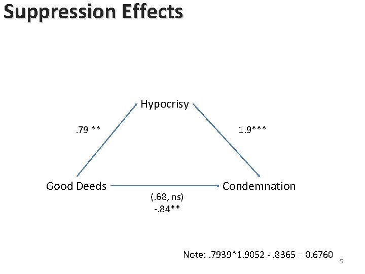
Suppression Effects Hypocrisy. 79 ** Good Deeds 1. 9*** (. 68, ns). 68, ns -. 84** Condemnation Note: . 7939*1. 9052 -. 8365 = 0. 6760 5

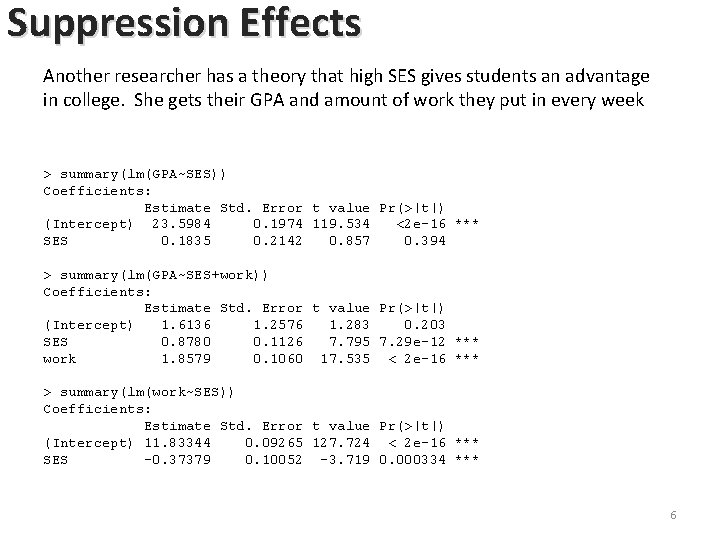
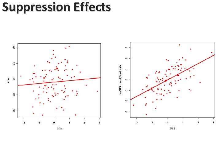
Suppression Effects Another researcher has a theory that high SES gives students an advantage in college. She gets their GPA and amount of work they put in every week > summary(lm(GPA~SES)) Coefficients: Estimate Std. Error t value Pr(>|t|) (Intercept) 23. 5984 0. 1974 119. 534 <2 e-16 *** SES 0. 1835 0. 2142 0. 857 0. 394 > summary(lm(GPA~SES+work)) Coefficients: Estimate Std. Error t value Pr(>|t|) (Intercept) 1. 6136 1. 2576 1. 283 0. 203 SES 0. 8780 0. 1126 7. 795 7. 29 e-12 *** work 1. 8579 0. 1060 17. 535 < 2 e-16 *** > summary(lm(work~SES)) Coefficients: Estimate Std. Error t value Pr(>|t|) (Intercept) 11. 83344 0. 09265 127. 724 < 2 e-16 *** SES -0. 37379 0. 10052 -3. 719 0. 000334 *** 6

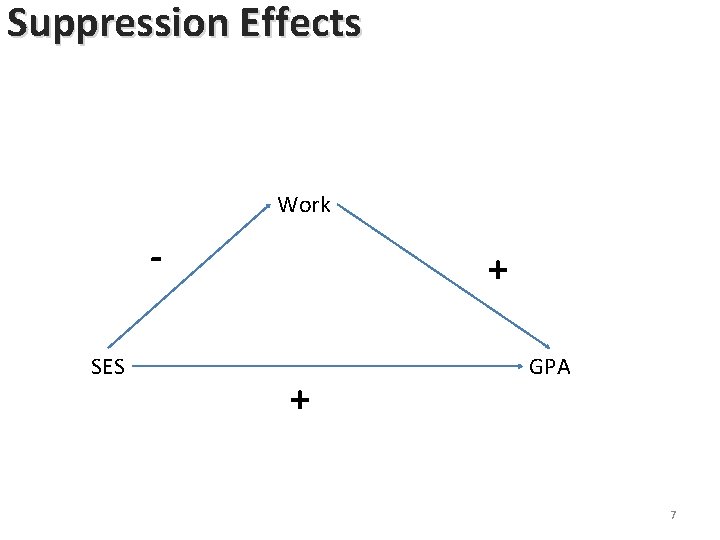
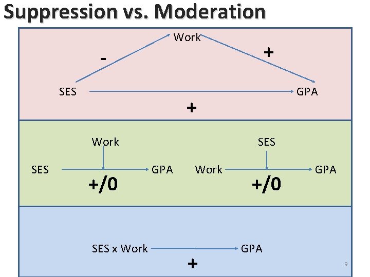
Suppression Effects Work SES + + + GPA 7

Suppression Effects

Suppression vs. Moderation Work + SES + Work SES GPA +/0 SES x Work SES GPA Work + +/0 GPA 9

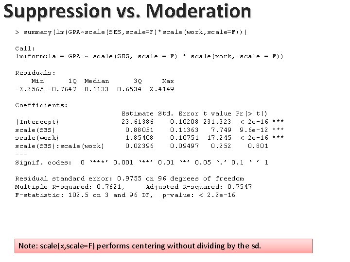
Suppression vs. Moderation > summary(lm(GPA~scale(SES, scale=F)*scale(work, scale=F))) Call: lm(formula = GPA ~ scale(SES, scale = F) * scale(work, scale = F)) Residuals: Min 1 Q -2. 2565 -0. 7647 Median 0. 1133 3 Q 0. 6534 Max 2. 4149 Coefficients: Estimate Std. Error t value Pr(>|t|) 23. 61386 0. 10208 231. 323 < 2 e-16 *** 0. 88051 0. 11363 7. 749 9. 6 e-12 *** 1. 85408 0. 10751 17. 245 < 2 e-16 *** 0. 02396 0. 09497 0. 252 0. 801 (Intercept) scale(SES) scale(work) scale(SES): scale(work) --Signif. codes: 0 ‘***’ 0. 001 ‘**’ 0. 01 ‘*’ 0. 05 ‘. ’ 0. 1 ‘ ’ 1 Residual standard error: 0. 9755 on 96 degrees of freedom Multiple R-squared: 0. 7621, Adjusted R-squared: 0. 7547 F-statistic: 102. 5 on 3 and 96 DF, p-value: < 2. 2 e-16 Note: scale(x, scale=F) performs centering without dividing by the sd.

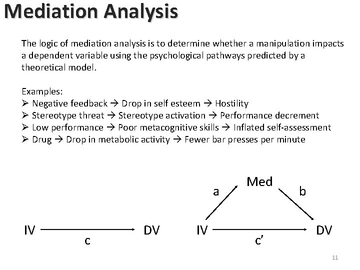
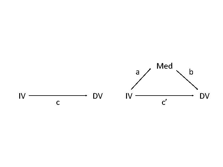
Mediation Analysis The logic of mediation analysis is to determine whether a manipulation impacts a dependent variable using the psychological pathways predicted by a theoretical model. Examples: Ø Negative feedback Drop in self esteem Hostility Ø Stereotype threat Stereotype activation Performance decrement Ø Low performance Poor metacognitive skills Inflated self-assessment Ø Drug Drop in metabolic activity Fewer bar presses per minute a IV c DV IV Med c’ b DV 11

Baron & Kenny (1986) Run three regressions: 1. DV = c IV + Intercept Gives you c 2. Med = a IV + Intercept Gives you a 3. DV = c’ IV + b Med + Intercept Gives you c’ and b Then four conditions have to be met to claim mediation: 1. c must be significant (that’s your original effect) 2. a must be significant 3. b must be significant 4. c’ must be reduced Test reduction (e. g. Sobel test) Complete vs. partial mediation a IV c DV IV Med c’ b DV 12

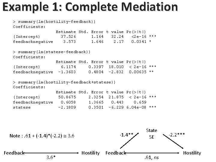
Example 1: Complete Mediation > summary(lm(hostility~feedback)) Coefficients: Estimate Std. Error t value Pr(>|t|) (Intercept) 37. 526 1. 164 32. 24 <2 e-16 *** feedbacknegative 3. 573 1. 646 2. 17 0. 0341 * > summary(lm(statese~feedback)) Coefficients: Estimate Std. Error t value Pr(>|t|) (Intercept) 6. 1174 0. 3397 18. 010 < 2 e-16 *** feedbacknegative -1. 3603 0. 4804 -2. 832 0. 00635 ** > summary(lm(hostility~feedback+statese)) Coefficients: Estimate Std. Error t value Pr(>|t|) (Intercept) 50. 8675 2. 3254 21. 875 < 2 e-16 *** feedbacknegative 0. 6058 1. 3665 0. 443 0. 659 statese -2. 1809 0. 3501 -6. 229 6. 04 e-08 *** -1. 4** Note : . 61 + (-1. 4)*(-2. 2) 3. 6 Feedback 3. 6* Hostility Feedback State SE . 61, ns -2. 2*** Hostility 13

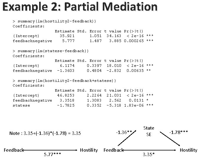
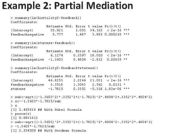
Example 2: Partial Mediation > summary(lm(hostility 2~feedback)) Coefficients: Estimate Std. Error t value Pr(>|t|) (Intercept) 35. 921 1. 051 34. 163 < 2 e-16 *** feedbacknegative 5. 777 1. 487 3. 885 0. 000265 *** > summary(lm(statese~feedback)) Coefficients: Estimate Std. Error t value Pr(>|t|) (Intercept) 6. 1174 0. 3397 18. 010 < 2 e-16 *** feedbacknegative -1. 3603 0. 4804 -2. 832 0. 00635 ** > summary(lm(hostility 2~feedback+statese)) Coefficients: Estimate Std. Error t value Pr(>|t|) (Intercept) 46. 8253 2. 2264 21. 031 < 2 e-16 *** feedbacknegative 3. 3518 1. 3083 2. 562 0. 0131 * statese -1. 7825 0. 3352 -5. 318 1. 83 e-06 *** Note : 3. 35+(-1. 36)*(-1. 78) = 3. 35 Feedback 5. 77*** Hostility -1. 36** Feedback State SE 3. 35* -1. 78*** Hostility 14

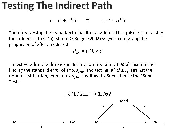
Testing The Indirect Path c = c’ + a*b c-c’ = a*b Therefore testing the reduction in the direct path (c-c’) is equivalent to testing the indirect path (a*b). Shrout & Bolger (2002) suggest computing the proportion of effect mediated: PM = a*b / c To test whether the drop is significant, Baron & Kenny (1986) recommend finding the standard error of a*b, sa*b, and testing (a*b/ sa*b) against the normal distribution, computing sa*b as defined by Sobel, hence the “Sobel Test. ” | a*b/ sa*b | > 1. 96? a IV c DV IV Med c’ b DV 15

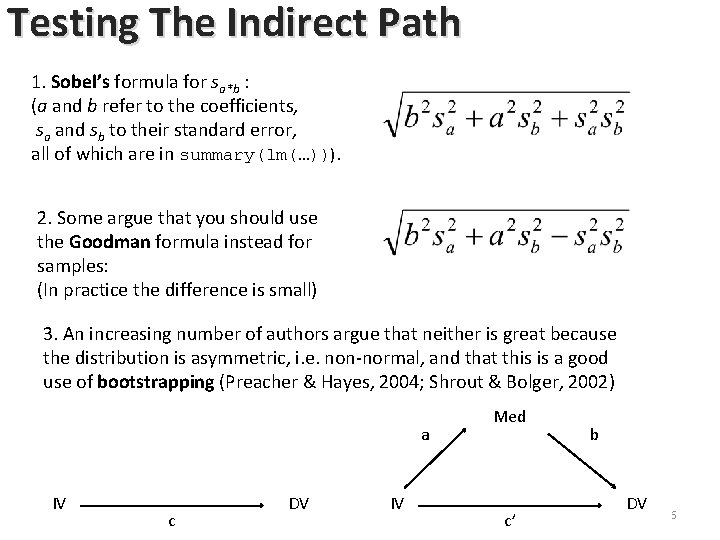
Testing The Indirect Path 1. Sobel’s formula for sa*b : (a and b refer to the coefficients, sa and sb to their standard error, all of which are in summary(lm(…))). 2. Some argue that you should use the Goodman formula instead for samples: (In practice the difference is small) 3. An increasing number of authors argue that neither is great because the distribution is asymmetric, i. e. non-normal, and that this is a good use of bootstrapping (Preacher & Hayes, 2004; Shrout & Bolger, 2002) a IV c DV IV Med c’ b DV 16

Example 2: Partial Mediation > summary(lm(hostility 2~feedback)) Coefficients: Estimate Std. Error t value Pr(>|t|) (Intercept) 35. 921 1. 051 34. 163 < 2 e-16 *** feedbacknegative 5. 777 1. 487 3. 885 0. 000265 *** > summary(lm(statese~feedback)) Coefficients: Estimate Std. Error t value Pr(>|t|) (Intercept) 6. 1174 0. 3397 18. 010 < 2 e-16 *** feedbacknegative -1. 3603 0. 4804 -2. 832 0. 00635 ** > summary(lm(hostility 2~feedback+statese)) Coefficients: Estimate Std. Error t value Pr(>|t|) (Intercept) 46. 8253 2. 2264 21. 031 < 2 e-16 *** feedbacknegative 3. 3518 1. 3083 2. 562 0. 0131 * statese -1. 7825 0. 3352 -5. 318 1. 83 e-06 *** > sab<-sqrt((-1. 3603^2)*. 3352^2+(-1. 7825)^2*. 4804^2+. 3352^2*. 4804^2) > z<--1. 3603*-1. 7825/sab > z [1] 2. 465616 ## With Sobel formula > pnorm(z) [1] 0. 9931611 > sab<-sqrt((-1. 3603)^2*. 3352^2+(-1. 7825)^2*. 4804^2 -. 3352^2*. 4804^2) > -1. 3603*-1. 7825/sab [1] 2. 534509 ## With Goodman formula

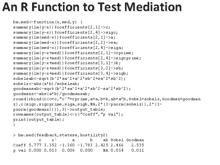
An R Function to Test Mediation bm. med<-function(x, med, y) { summary(lm(y~x))$coefficients[2, 1]->c; summary(lm(y~x))$coefficients[2, 4]->sigc; summary(lm(med~x))$coefficients[2, 1]->a; summary(lm(med~x))$coefficients[2, 2]->sa; summary(lm(med~x))$coefficients[2, 4]->siga; summary(lm(y~x+med))$coefficients[2, 1]->cprime; summary(lm(y~x+med))$coefficients[2, 4]->sigcprime; summary(lm(y~x+med))$coefficients[3, 1]->b; summary(lm(y~x+med))$coefficients[3, 2]->sb; summary(lm(y~x+med))$coefficients[3, 4]->sigb; sobelsab<-sqrt(b^2*sa^2+a^2*sb^2+sa^2*sb^2); sobelz<-abs(a*b)/sobelsab; goodmansab<-sqrt(b^2*sa^2+a^2*sb^2 -sa^2*sb^2); goodmanz<-abs(a*b)/goodmansab; round(rbind(c(c=c, "c'"=cprime, a=a, b=b, ab=a*b, Sobel=sobelz, Goodman=goodman z), c(sigc, sigcprime, siga, sigb, NA, 2*(1 -pnorm(sobelz)), 2*(1 pnorm(goodmanz)))), 3)->output_table; rownames(output_table)<-c("Coeff", "p val"); print(output_table); } > bm. med(feedback, statese, hostility 2) c c' a b ab Sobel Goodman Coeff 5. 777 3. 352 -1. 360 -1. 783 2. 425 2. 466 2. 535 p val 0. 000 0. 013 0. 006 0. 000 NA 0. 014 0. 011

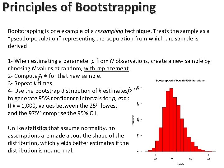
Principles of Bootstrapping is one example of a resampling technique. Treats the sample as a “pseudo-population” representing the population from which the sample is derived. 1 - When estimating a parameter p from N observations, create a new sample by choosing N values at random, with replacement. 2 - Compute for that new sample. 3 - Repeat k times. 4 - Use the bootstrap distribution of k estimates to generate 95% confidence intervals for p, etc. : If k = 1, 000, values between the 25 th lowest and the 975 th comprise the 95% C. I. Unlike statistics that assume normality, no assumptions are made about the shape of the distribution, which yields better estimates if the distribution is not normal.

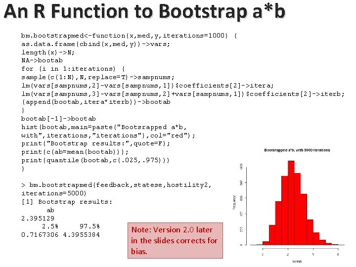
An R Function to Bootstrap a*b bm. bootstrapmed<-function(x, med, y, iterations=1000) { as. data. frame(cbind(x, med, y))->vars; length(x)->N; NA->bootab for (i in 1: iterations) { sample(c(1: N), N, replace=T)->sampnums; lm(vars[sampnums, 2]~vars[sampnums, 1])$coefficients[2]->itera; lm(vars[sampnums, 3]~vars[sampnums, 2]+vars[sampnums, 1])$coefficients[2]->iterb; (append(bootab, itera*iterb))->bootab } bootab[-1]->bootab hist(bootab, main=paste("Bootsrapped a*b, with", iterations, "iterations"), col="red"); print("Bootstrap results: ", quote=F); print(c(ab=mean(bootab))); print(quantile(bootab, c(. 025, . 975))) } > bm. bootstrapmed(feedback, statese, hostility 2, iterations=5000) [1] Bootstrap results: ab 2. 395129 2. 5% 97. 5% Note: Version 2. 0 later 0. 7167306 4. 3955384 in the slides corrects for bias.

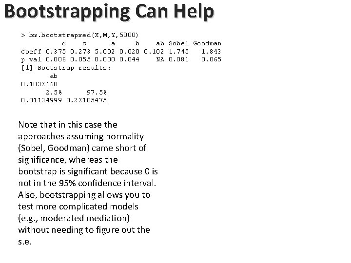
Bootstrapping Can Help > bm. bootstrapmed(X, M, Y, 5000) c c' a b ab Sobel Goodman Coeff 0. 375 0. 273 5. 002 0. 020 0. 102 1. 745 1. 843 p val 0. 006 0. 055 0. 000 0. 044 NA 0. 081 0. 065 [1] Bootstrap results: ab 0. 1032160 2. 5% 97. 5% 0. 01134999 0. 22105475 Note that in this case the approaches assuming normality (Sobel, Goodman) came short of significance, whereas the bootstrap is significant because 0 is not in the 95% confidence interval. Also, bootstrapping allows you to test more complicated models (e. g. , moderated mediation) without needing to figure out the s. e.

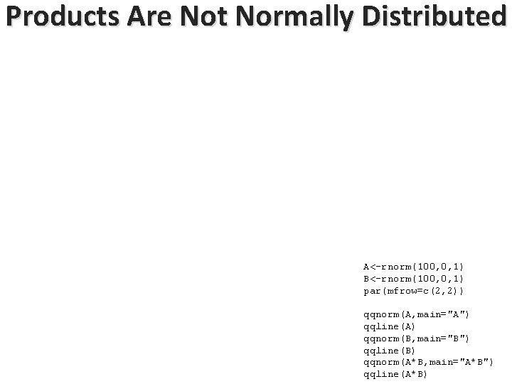
Products Are Not Normally Distributed A<-rnorm(100, 0, 1) B<-rnorm(100, 0, 1) par(mfrow=c(2, 2)) qqnorm(A, main="A") qqline(A) qqnorm(B, main="B") qqline(B) qqnorm(A*B, main="A*B") qqline(A*B)

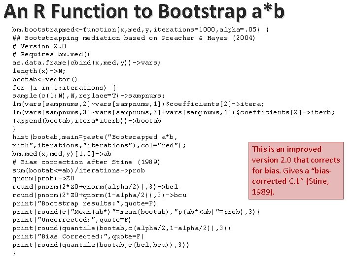
An R Function to Bootstrap a*b bm. bootstrapmed<-function(x, med, y, iterations=1000, alpha=. 05) { ## Bootstrapping mediation based on Preacher & Hayes (2004) # Version 2. 0 # Requires bm. med() as. data. frame(cbind(x, med, y))->vars; length(x)->N; bootab<-vector() for (i in 1: iterations) { sample(c(1: N), N, replace=T)->sampnums; lm(vars[sampnums, 2]~vars[sampnums, 1])$coefficients[2]->itera; lm(vars[sampnums, 3]~vars[sampnums, 2]+vars[sampnums, 1])$coefficients[2]->iterb; (append(bootab, itera*iterb))->bootab } hist(bootab, main=paste("Bootsrapped a*b, with", iterations, "iterations"), col="red"); This is an improved bm. med(x, med, y)[1, 5]->ab version 2. 0 that corrects # Bias correction after Stine (1989) sum(bootab<=ab)/iterations->prob for bias. Gives a “biasqnorm(prob)->Z 0 corrected C. I. ” (Stine, round(pnorm(2*Z 0+qnorm(alpha/2)), 3)->bcl 1989). round(pnorm(2*Z 0+qnorm(1 -alpha/2)), 3)->bcu print("Bootstrap results: ", quote=F) print(round(c("Mean(ab*)"=mean(bootab), "p(ab*<ab)"=prob), 3)) print("Uncorrected: ", quote=F) print(round(quantile(bootab, c(alpha/2, 1 -alpha/2)), 3)) print("Bias Corrected: ", quote=F) print(round(quantile(bootab, c(bcl, bcu)), 3)) }

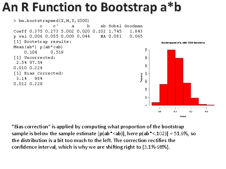
An R Function to Bootstrap a*b > bm. bootstrapmed(X, M, Y, 1000) c c' a b ab Sobel Goodman Coeff 0. 375 0. 273 5. 002 0. 020 0. 102 1. 745 1. 843 p val 0. 006 0. 055 0. 000 0. 044 NA 0. 081 0. 065 [1] Bootstrap results: Mean(ab*) p(ab*<ab) 0. 104 0. 519 [1] Uncorrected: 2. 5% 97. 5% 0. 010 0. 224 [1] Bias Corrected: 3. 1% 98% 0. 012 0. 229 “Bias correction” is applied by computing what proportion of the bootstrap sample is below the sample estimate [p(ab*<ab)], here p(ab*<. 102)] = 51. 9%, so the distribution is a bit too much to the left. The correction rectifies the confidence interval, which is why we are shifting right to {3. 1%-98%}.

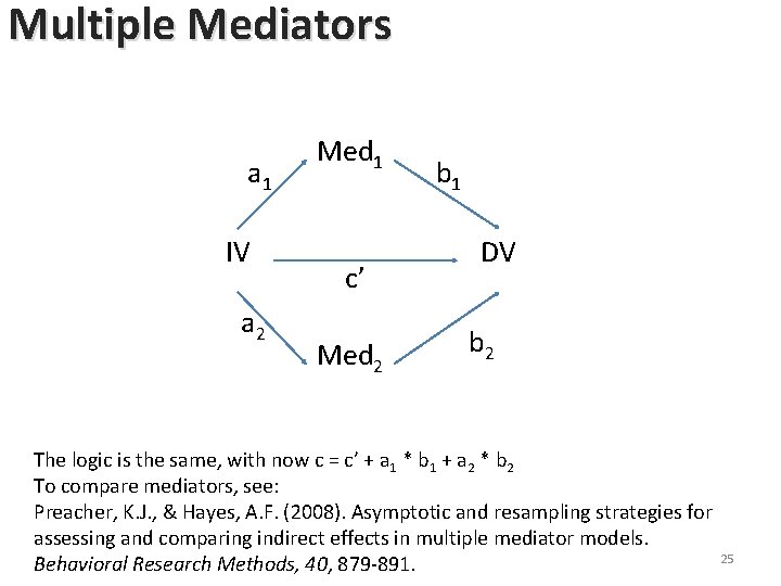
Multiple Mediators a 1 IV a 2 Med 1 c’ Med 2 b 1 DV b 2 The logic is the same, with now c = c’ + a 1 * b 1 + a 2 * b 2 To compare mediators, see: Preacher, K. J. , & Hayes, A. F. (2008). Asymptotic and resampling strategies for assessing and comparing indirect effects in multiple mediator models. 25 Behavioral Research Methods, 40, 879 -891.

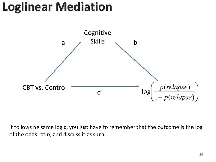
Loglinear Mediation a CBT vs. Control Cognitive Skills c’ b Relapse ? (YES /NO) It follows he same logic, you just have to remember that the outcome is the log of the odds ratio, and discuss it as such. 26

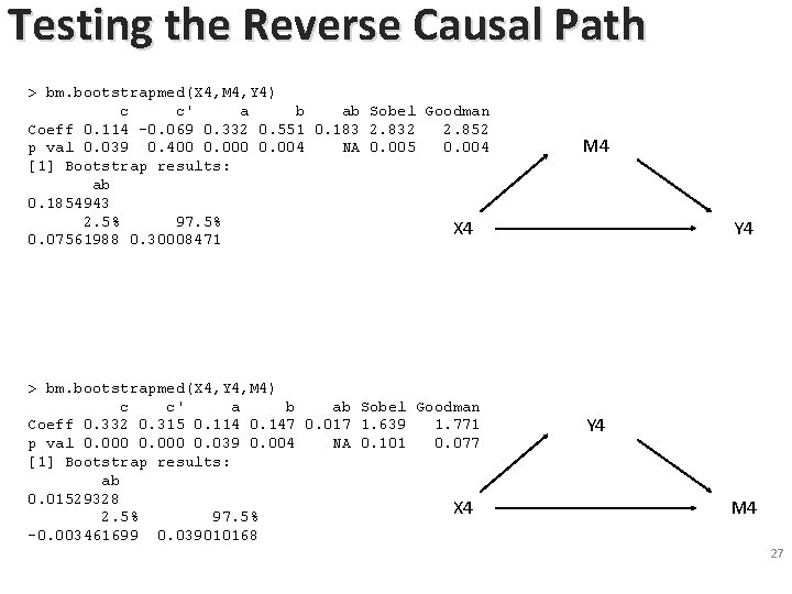
Testing the Reverse Causal Path > bm. bootstrapmed(X 4, M 4, Y 4) c c' a b ab Sobel Goodman Coeff 0. 114 -0. 069 0. 332 0. 551 0. 183 2. 832 2. 852 p val 0. 039 0. 400 0. 004 NA 0. 005 0. 004 [1] Bootstrap results: ab 0. 1854943 2. 5% 97. 5% X 4 0. 07561988 0. 30008471 > bm. bootstrapmed(X 4, Y 4, M 4) c c' a b ab Sobel Goodman Coeff 0. 332 0. 315 0. 114 0. 147 0. 017 1. 639 1. 771 p val 0. 000 0. 039 0. 004 NA 0. 101 0. 077 [1] Bootstrap results: ab 0. 01529328 X 4 2. 5% 97. 5% -0. 003461699 0. 039010168 M 4 Y 4 27 M 4 27 Y 4 27

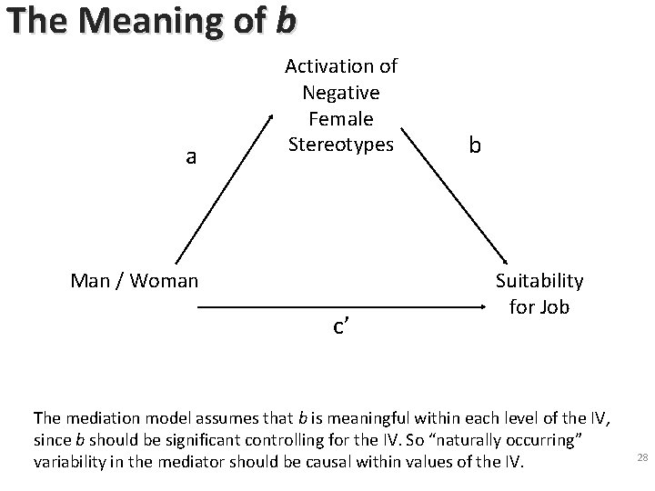
The Meaning of b a Activation of Negative Female Stereotypes Man / Woman c’ b Suitability for Job The mediation model assumes that b is meaningful within each level of the IV, since b should be significant controlling for the IV. So “naturally occurring” variability in the mediator should be causal within values of the IV. 28

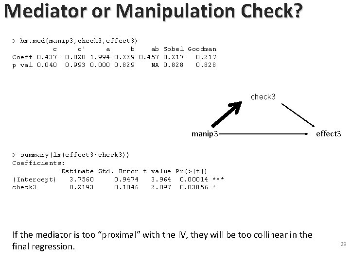
Mediator or Manipulation Check? > bm. med(manip 3, check 3, effect 3) c c' a b ab Sobel Goodman Coeff 0. 437 -0. 020 1. 994 0. 229 0. 457 0. 217 p val 0. 040 0. 993 0. 000 0. 829 NA 0. 828 check 3 manip 3 effect 329 > summary(lm(effect 3~check 3)) Coefficients: Estimate Std. Error t value Pr(>|t|) (Intercept) 3. 7560 0. 9474 3. 964 0. 00014 *** check 3 0. 2193 0. 1046 2. 097 0. 03856 * If the mediator is too “proximal” with the IV, they will be too collinear in the final regression. 29

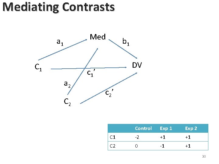
Mediating Contrasts Med a 1 C 1 a 2 C 2 b 1 DV c 1’ c 2’ Control Exp 1 Exp 2 C 1 -2 +1 +1 C 2 0 -1 +1 30

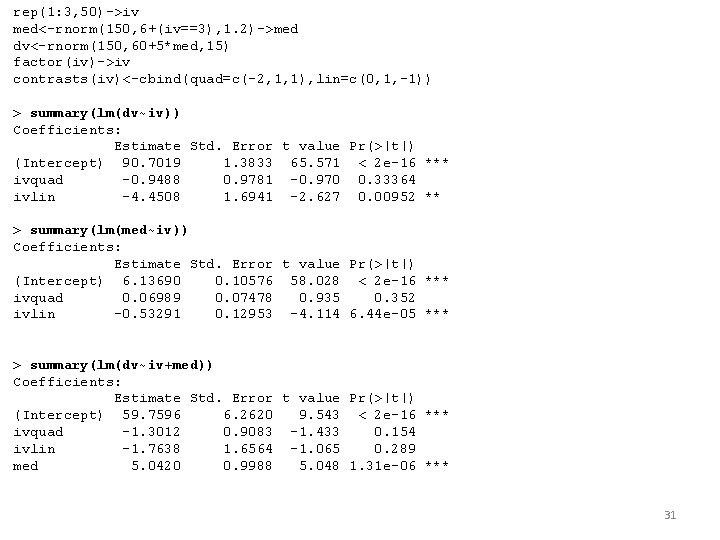
rep(1: 3, 50)->iv med<-rnorm(150, 6+(iv==3), 1. 2)->med dv<-rnorm(150, 60+5*med, 15) factor(iv)->iv contrasts(iv)<-cbind(quad=c(-2, 1, 1), lin=c(0, 1, -1)) > summary(lm(dv~iv)) Coefficients: Estimate Std. Error t value Pr(>|t|) (Intercept) 90. 7019 1. 3833 65. 571 < 2 e-16 *** ivquad -0. 9488 0. 9781 -0. 970 0. 33364 ivlin -4. 4508 1. 6941 -2. 627 0. 00952 ** > summary(lm(med~iv)) Coefficients: Estimate Std. Error t value Pr(>|t|) (Intercept) 6. 13690 0. 10576 58. 028 < 2 e-16 *** ivquad 0. 06989 0. 07478 0. 935 0. 352 ivlin -0. 53291 0. 12953 -4. 114 6. 44 e-05 *** > summary(lm(dv~iv+med)) Coefficients: Estimate Std. Error t value Pr(>|t|) (Intercept) 59. 7596 6. 2620 9. 543 < 2 e-16 *** ivquad -1. 3012 0. 9083 -1. 433 0. 154 ivlin -1. 7638 1. 6564 -1. 065 0. 289 med 5. 0420 0. 9988 5. 048 1. 31 e-06 *** 31

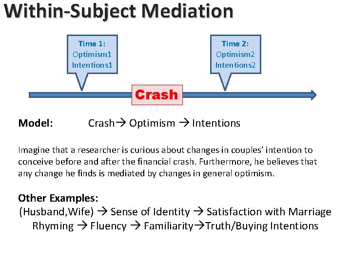
Within-Subject Mediation Time 1: Optimism 1 Intentions 1 Time 2: Optimism 2 Intentions 2 Crash Model: Crash Optimism Intentions Imagine that a researcher is curious about changes in couples’ intention to conceive before and after the financial crash. Furthermore, he believes that any change he finds is mediated by changes in general optimism. Other Examples: (Husband, Wife) Sense of Identity Satisfaction with Marriage Rhyming Fluency Familiarity Truth/Buying Intentions

a IV c DV IV Med c’ b DV

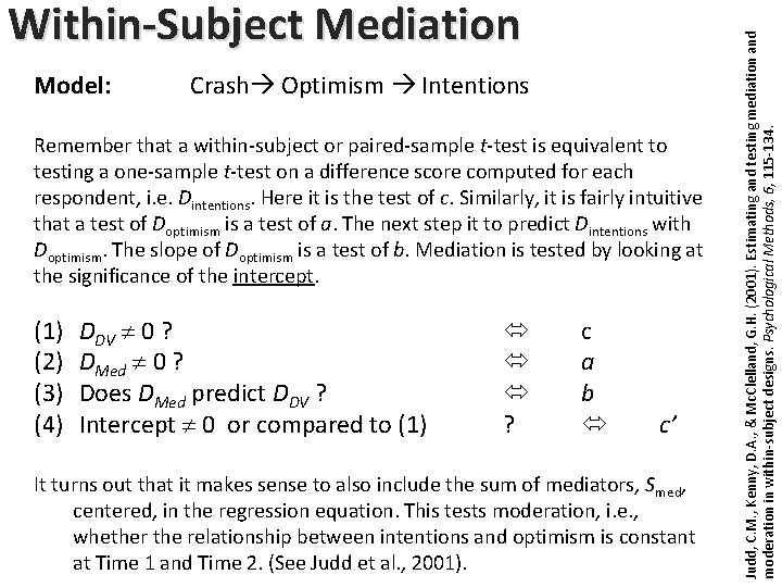
Model: Crash Optimism Intentions Remember that a within-subject or paired-sample t-test is equivalent to testing a one-sample t-test on a difference score computed for each respondent, i. e. Dintentions. Here it is the test of c. Similarly, it is fairly intuitive that a test of Doptimism is a test of a. The next step it to predict Dintentions with Doptimism. The slope of Doptimism is a test of b. Mediation is tested by looking at the significance of the intercept. (1) (2) (3) (4) DDV 0 ? DMed 0 ? Does DMed predict DDV ? Intercept 0 or compared to (1) ? c a b c’ It turns out that it makes sense to also include the sum of mediators, Smed, centered, in the regression equation. This tests moderation, i. e. , whether the relationship between intentions and optimism is constant at Time 1 and Time 2. (See Judd et al. , 2001). Judd, C. M. , Kenny, D. A. , & Mc. Clelland, G. H. (2001). Estimating and testing mediation and moderation in within-subject designs. Psychological Methods, 6, 115 -134. Within-Subject Mediation

Within-Subject Mediation: Example 1

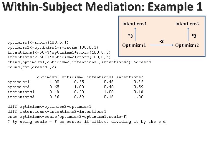
Within-Subject Mediation: Example 1 Intentions 1 *3 optimism 1<-rnorm(100, 5, 1) Optimism 1 optimism 2<-optimism 1 -2+rnorm(100, 0, 1) intentions 1<-50+3*optimism 1+rnorm(100, 0, 5) intentions 2<-50+3*optimism 2+rnorm(100, 0, 5) cbind(optimism 1, optimism 2, intentions 1, intentions 2)->crashd round(cor(crashd), 2) Intentions 2 -2 optimism 1 optimism 2 intentions 1 intentions 2 optimism 1 1. 00 0. 65 0. 48 0. 36 optimism 2 0. 65 1. 00 0. 40 0. 59 intentions 1 0. 48 0. 40 1. 00 0. 18 intentions 2 0. 36 0. 59 0. 18 1. 00 diff_optimism<-optimism 2 -optimism 1 diff_intentions<-intentions 2 -intentions 1 csum_optimism<-scale(optimism 2+optimism 1, scale=F) # By using scale = F we center it without dividing it by the s. d. *3 Optimism 2

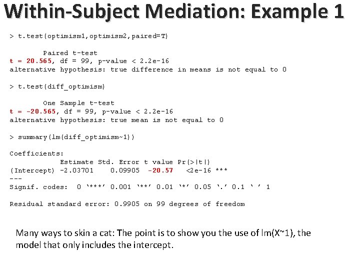
Within-Subject Mediation: Example 1 > t. test(optimism 1, optimism 2, paired=T) Paired t-test t = 20. 565, df = 99, p-value < 2. 2 e-16 alternative hypothesis: true difference in means is not equal to 0 > t. test(diff_optimism) One Sample t-test t = -20. 565, df = 99, p-value < 2. 2 e-16 alternative hypothesis: true mean is not equal to 0 > summary(lm(diff_optimism~1)) Coefficients: Estimate Std. Error t value Pr(>|t|) (Intercept) -2. 03701 0. 09905 -20. 57 <2 e-16 *** --Signif. codes: 0 ‘***’ 0. 001 ‘**’ 0. 01 ‘*’ 0. 05 ‘. ’ 0. 1 ‘ ’ 1 Residual standard error: 0. 9905 on 99 degrees of freedom Many ways to skin a cat: The point is to show you the use of lm(X~1), the model that only includes the intercept.

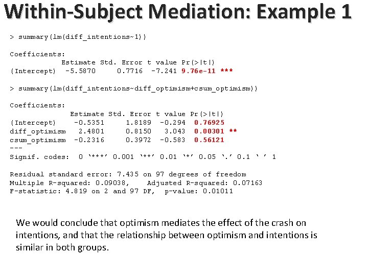
Within-Subject Mediation: Example 1 > summary(lm(diff_intentions~1)) Coefficients: Estimate Std. Error t value Pr(>|t|) (Intercept) -5. 5870 0. 7716 -7. 241 9. 76 e-11 *** > summary(lm(diff_intentions~diff_optimism+csum_optimism)) Coefficients: Estimate Std. Error t value Pr(>|t|) (Intercept) -0. 5351 1. 8189 -0. 294 0. 76925 diff_optimism 2. 4801 0. 8150 3. 043 0. 00301 ** csum_optimism -0. 2316 0. 3972 -0. 583 0. 56121 --Signif. codes: 0 ‘***’ 0. 001 ‘**’ 0. 01 ‘*’ 0. 05 ‘. ’ 0. 1 ‘ ’ 1 Residual standard error: 7. 435 on 97 degrees of freedom Multiple R-squared: 0. 09038, Adjusted R-squared: 0. 07163 F-statistic: 4. 819 on 2 and 97 DF, p-value: 0. 01011 We would conclude that optimism mediates the effect of the crash on intentions, and that the relationship between optimism and intentions is similar in both groups.

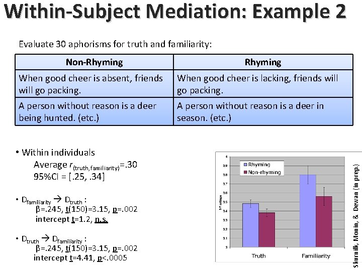
Within-Subject Mediation: Example 2 Evaluate 30 aphorisms for truth and familiarity: Rhyming When good cheer is absent, friends will go packing. When good cheer is lacking, friends will go packing. A person without reason is a deer being hunted. (etc. ) A person without reason is a deer in season. (etc. ) • Within individuals Average r(truth, familiarity)=. 30 95%CI = [. 25, . 34] • Dfamiliarity Dtruth : β=. 245, t(150)=3. 15, p=. 002 intercept t=1. 2, n. s. • Dtruth Dfamiliarity : β=. 245, t(150)=3. 15, p=. 002 intercept t=4. 41, p<. 0005 Skurnilk, Monin, & Dewan (in prep. ) Non-Rhyming

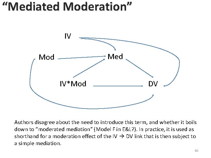
“Mediated Moderation” IV Med Mod IV*Mod DV Authors disagree about the need to introduce this term, and whether it boils down to “moderated mediation” (Model F in E&L? ). In practice, it is used as shorthand for a moderation effect of the IV DV link that is then subject to a simple mediation. 40

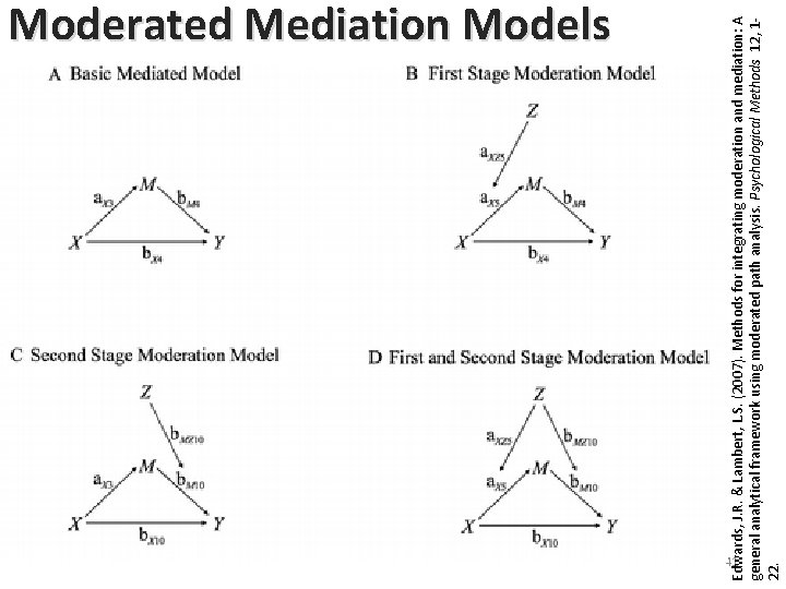
41 Edwards, J. R. & Lambert, L. S. (2007). Methods for integrating moderation and mediation: A general analytical framework using moderated path analysis. Psychological Methods 12, 122. Moderated Mediation Models

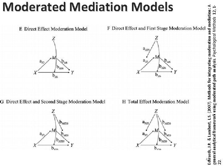
42 Edwards, J. R. & Lambert, L. S. (2007). Methods for integrating moderation and mediation: A general analytical framework using moderated path analysis. Psychological Methods 12, 122. Moderated Mediation Models

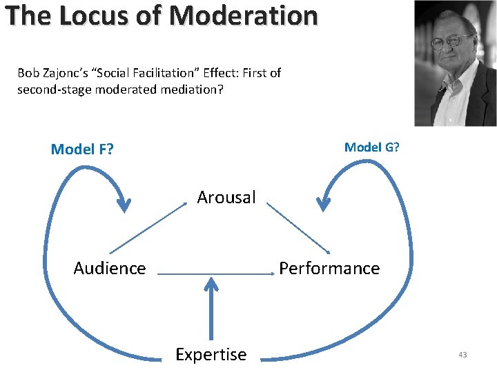
The Locus of Moderation Bob Zajonc’s “Social Facilitation” Effect: First of second-stage moderated mediation? Model F? Model G? Arousal Audience Performance Expertise 43

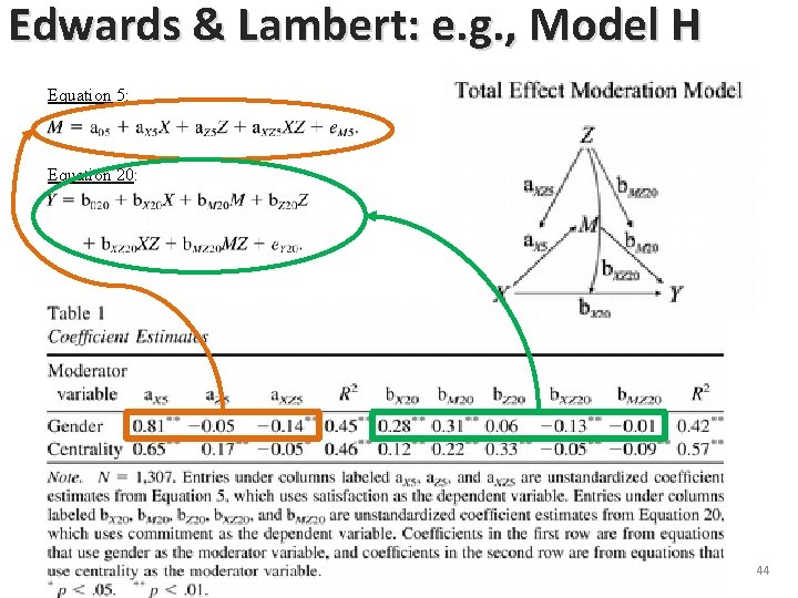
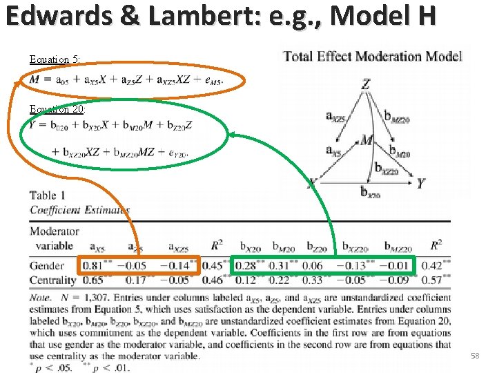
Edwards & Lambert: e. g. , Model H Equation 5: Equation 20: 44

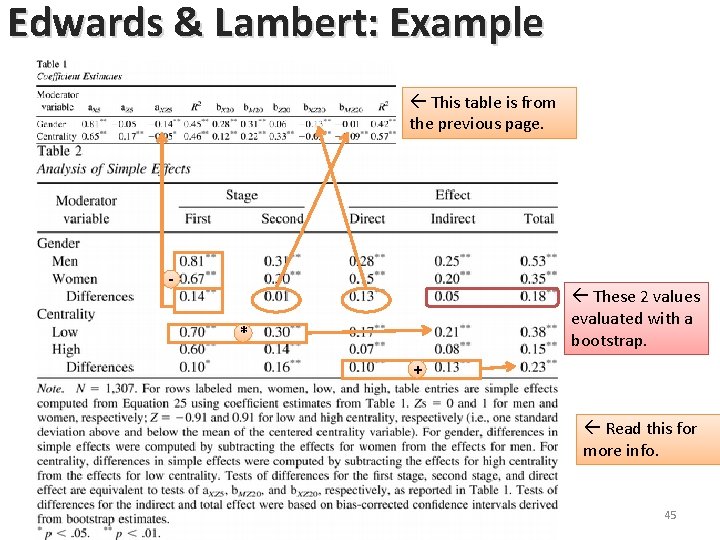
Edwards & Lambert: Example This table is from the previous page. - These 2 values evaluated with a bootstrap. * + Read this for more info. 45

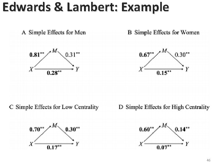
Edwards & Lambert: Example 46

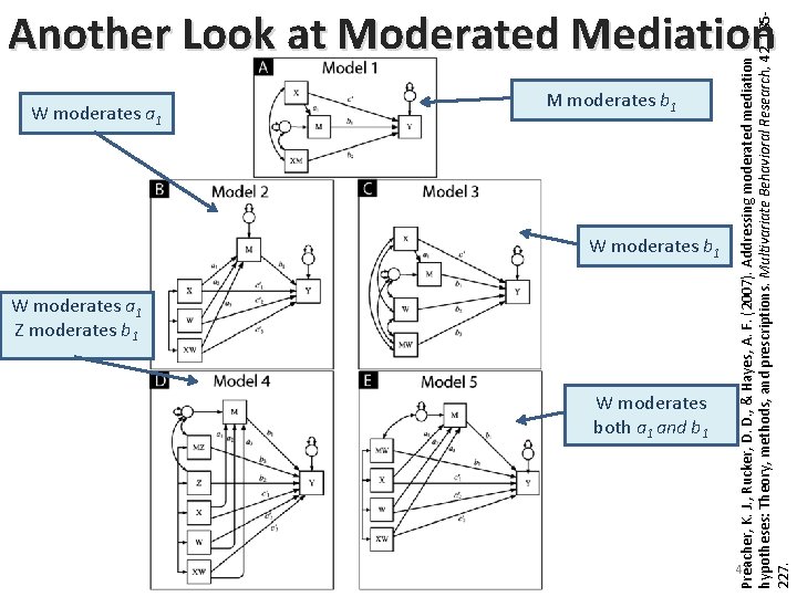
W moderates a 1 M moderates b 1 W moderates a 1 Z moderates b 1 W moderates both a 1 and b 1 47 Preacher, K. J. , Rucker, D. D. , & Hayes, A. F. (2007). Addressing moderated mediation hypotheses: Theory, methods, and prescriptions. Multivariate Behavioral Research, 42, 185227. Another Look at Moderated Mediation

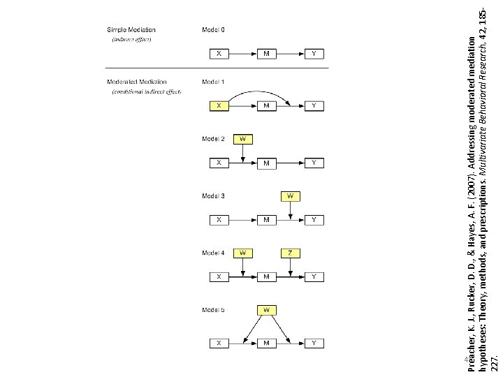
Preacher, K. J. , Rucker, D. D. , & Hayes, A. F. (2007). Addressing moderated mediation hypotheses: Theory, methods, and prescriptions. Multivariate Behavioral Research, 42, 185227. 48

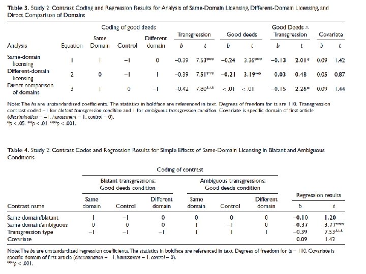
49

50

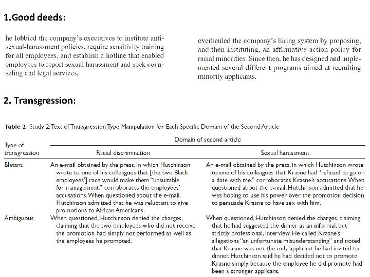
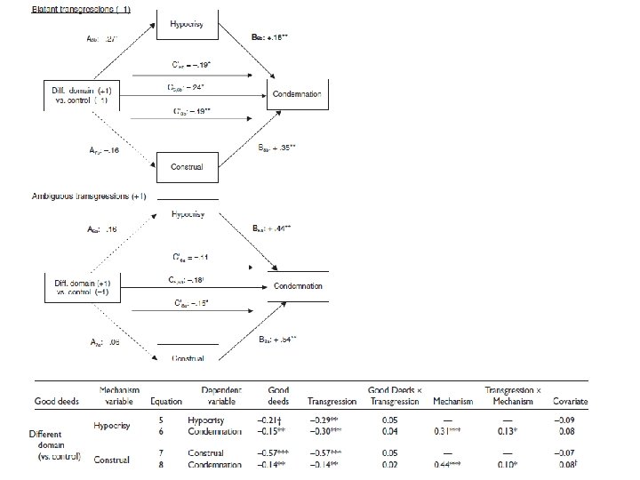
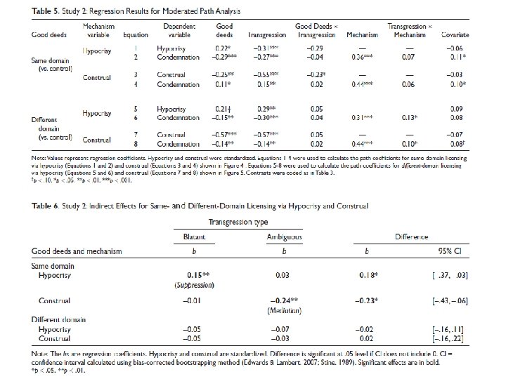
1. Good deeds: 2. Transgression: 51

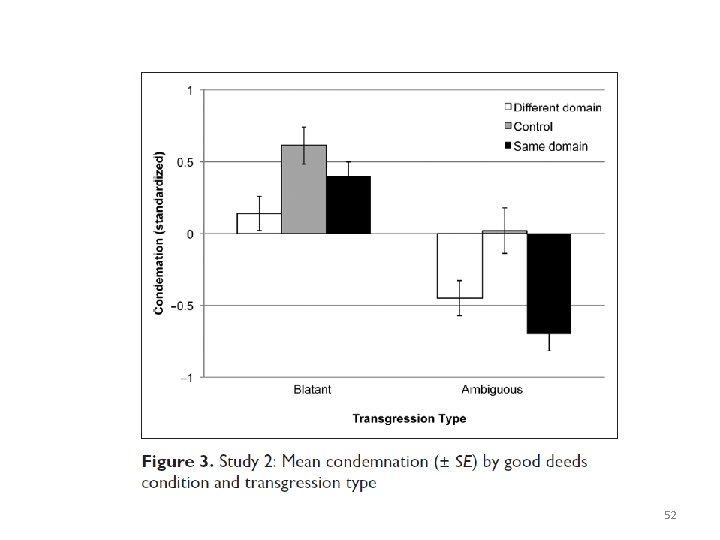
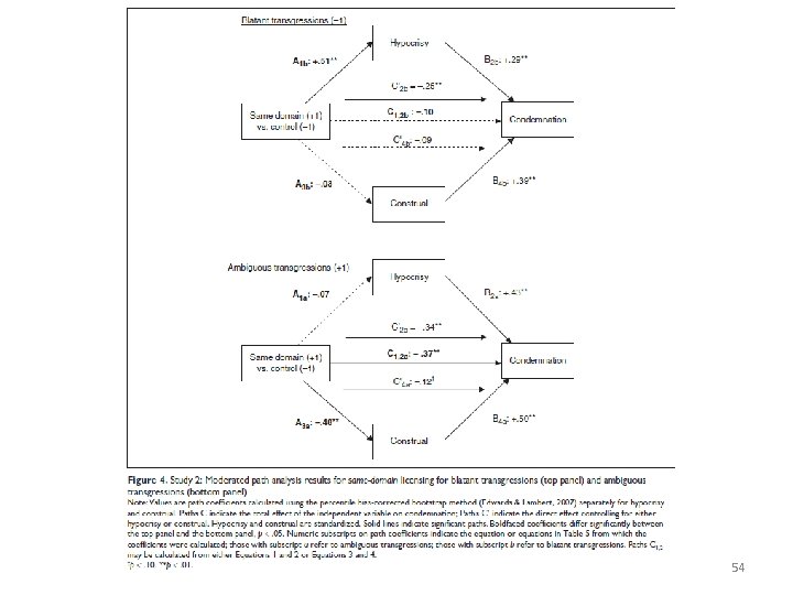
52

53

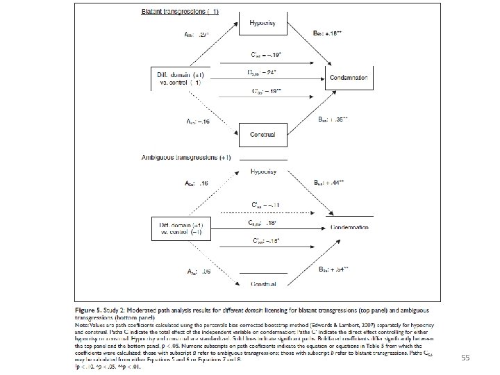
54

55

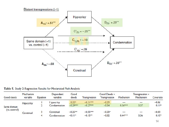
56

57

Edwards & Lambert: e. g. , Model H Equation 5: Equation 20: 58

59

References Baron, R. M. , & Kenny, D. A. (1986). The moderator-mediator variable distinction in social psychological research: Conceptual, strategic, and statistical considerations. Journal of Personality and Social Psychology, 51, 1173 -1182. ## The original paper. These tend to advocate bootstrapping: Shrout, P. E. , & Bolger, N. (2002). Mediation in experimental and nonexperimental studies: New procedures and recommendations. Psychological Methods, 7, 422 -445. Mac. Kinnon, D. P. , Lockwood, C. M. , Hoffman, J. M. , West, S. G. , & Sheets, V. (2002). A comparison of methods to test mediation and other intervening variable effects. Psychological Methods, 7, 83 -104. Preacher, K. J. & Hayes, A. F. (2004). SPSS and SAS procedures for estimating indirect effects in simple mediation models. Behavior Research Methods, Instruments, and Computers, 36, 717 -731. ## A short technical paper – the other 2 are bigger reviews. Preacher, K. J. , & Hayes, A. F. (2008). Asymptotic and resampling strategies for assessing and comparing indirect effects in multiple mediator models. Behavioral Research Methods, 40, 879 -891. 60

References (cont. ) Moderated Mediation: Preacher, K. J. , Rucker, D. D. , & Hayes, A. F. (2007). Addressing moderated mediation hypotheses: Theory, methods, and prescriptions. Multivariate Behavioral Research, 42, 185 -227. Edwards, J. R. & Lambert, L. S. (2007). Methods for integrating moderation and mediation: A general analytical framework using moderated path analysis. Psychological Methods 12, 1 -22. ## My favorite of the three. Approaches Critical of Mediation: Sigall, H. & Mills, J. (1998). Measure of independent variables and mediators are useful in social psychology experiments: But are they necessary? Personality and Social Psychology Review, 2, 218226. Spencer, S. J. , Zanna, M. P. , & Fong, G. T. (2005). Establishing a causal chain: Why experiments are often more effective than mediational analyses in examining psychological processes. Journal of Personality and Social Psychology, 89, 845 -851. 61

References (cont. ) How to test mediation in within-subject designs: Judd, C. M. , Kenny, D. A. , & Mc. Clelland, G. H. (2001). Estimating and testing mediation and moderation in within-subject designs. Psychological Methods, 6, 115 -134. A Good Introduction to Bootstrapping (Also Discusses Bias Correction): Stine, R. (1989). An introduction to bootstrap methods: Examples & ideas. Sociological Methods & Research, 18, 243 -291. 62

Which Test To Use? 63

1. You want to see whether men and women change their political attitudes differently throughout college. You follow a group of 50 men and 50 women for four years, and in September of their freshman, sophomore, junior and senior year they fill out political attitudes questionnaires. 2. You wonder if opposition to gay marriage is more prevalent in rural Californian counties, and if so, if it’s due to the influence of traditional religious values. For every county in California, you obtain a) estimates of church attendance, b) support for Prop. 8, and c) an index of urbanization. 3. You wonder whether a new cycling incentive will make people want to use their bike to work more. You survey a group of Stanford employees about their willingness (on a scale from 1 to 5) to bike to work before the incentives are put into place, and a week after the new incentives are advertised you survey another group of employees. 4. You wonder whether the incentives for biking are even working. You count the number of people you can count cycling on the Oval in a 10 -minute period at 10 am one week before the incentives are in place and one week after they are in place. 64

5. You are wondering how to improve the gas mileage on your brand new hybrid. Every time you fill the tank, you write down how much it’s rained since your last fill (0: not at all 3: all the time), how much time you’d estimate you spent on the highway (%), how much time you vs. your husband drove the car (%), how many miles you went (from the odometer), and how much tread is left on your tires (in mm). 6. You want to know the impact of chewing time on the size of gum bubbles. You divide your class of 90 students into three equal-sized groups: one group chews a fresh piece of gum for 10 seconds, one groups chews for 1 minute, and the third group chews for the entire one-hour class. Then you ask them to produce the biggest bubble possible, and you use NSF-funded laser technology that your adviser obtained to measure the volume of rat brains to measure the size of each bubble. To test whether brand matters, you grabbed one pack at the local grocery store from each of the 10 most popular kinds, and you made sure that 3 people in each group got to sample one of the 10. 7. You want to test the effect of alcohol on risky and non-risky behaviors. You survey a bunch of friends about their willingness to try out risky behavior vs. their willingness to try out non-risky behavior (you ask them to express both in percentages). A week later you gather the same friends at a party after they've 65 all had drinks and you ask them the same two questions.

8. You are interested in people’s ability to follow through with their exercising intentions. You get a list of joggers from a local running club, and send each a survey asking them how many hours they plan to jog in the next two weeks. Then unbeknownst to them you send undergraduate research assistants to spy on them for two weeks and record how many hours they actually went jogging. You wonder if the joggers’ intentions are in line with their behavior. 9. You compare the happiness with their commute of people who come to school by bike, car, train or foot. You only include in your study people who always use the same mode of transportation (for simplicity). You survey people as they get to school on sunny days and on rainy days, and you write that down. You also decide to separate people who come to school 4 or 5 days a week from people who don't come in as much. 10. You study the impact of contact on mother and teenage child satisfaction with the relationship. You get 30 mother-child dyads, and you get satisfaction ratings for each. Some of these dyads see each other all the time, others only see each other only on weekends. Additionally, you wonder if teenage and mother satisfaction are related. 66

11. You wonder if “Gay Blue Jeans Day” is getting more people to wear jeans (or fewer? ). You spend 15 minutes at Tressider counting how many people walk in the door and how many of them wear jeans and how many don’t. You do the same thing a week later. 12. A British friend of yours is always claiming that Americans don’t know World geography. Mildly offended and wanting to settle the score once and for all, you round up a sample of 30 US students and 28 European exchange students and record how many foreign countries they can name when shown a blank map. 13. You decide to study the impact of car value, attractiveness, and gender on whether someone gets a ticket after having been pulled over for making an illegal left turn. You know a corner where opportunistic motorcycle cops like to wait and watch them for a few days as they pulls people over. For each you record the variables above. You also suspect that attractive women get away, but attractive men don’t. In fact, you wonder if men in expensive cars are not more likely to get a ticket. 67