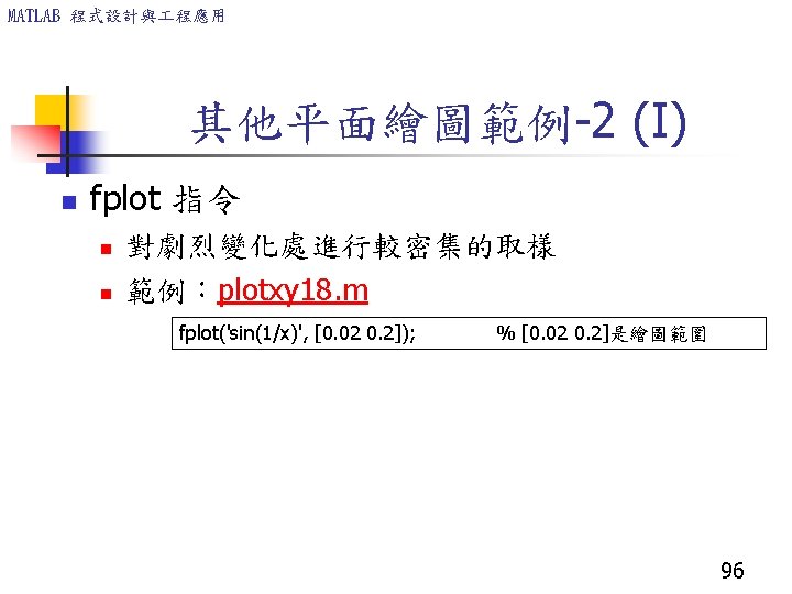
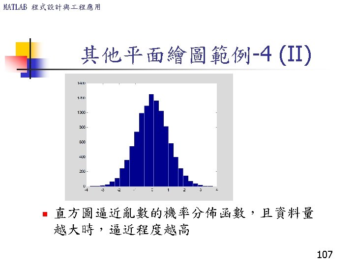
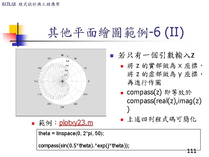
A complete plot w title axis labels legend

A complete plot w/ title, axis labels, legend, grid and multiple line styles MATLAB 程式設計與 程應用 2

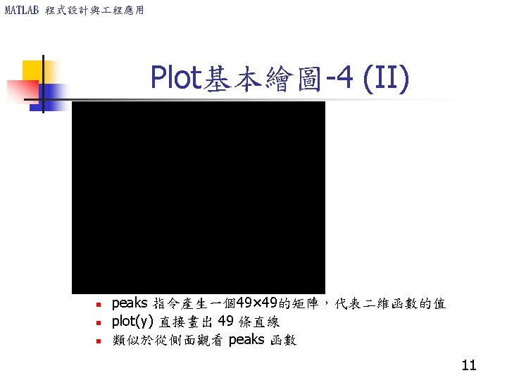

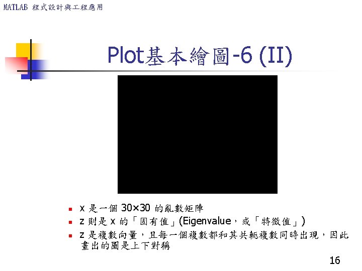
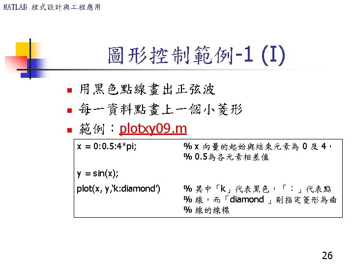
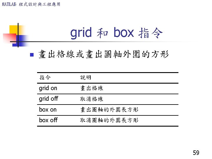
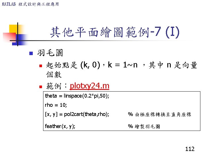
![MATLAB 程式設計與 程應用 Z=0. 1+0. 9 i; N=[0: 0. 1: 10]; Plot(z. ^n), xlabel(‘Real’),](http://slidetodoc.com/presentation_image/5995f4392edc9fef2052c101b58d3490/image-17.jpg "MATLAB 程式設計與 程應用 Z=0. 1+0. 9 i; N=[0: 0. 1: 10]; Plot(z. ^n), xlabel(‘Real’),")
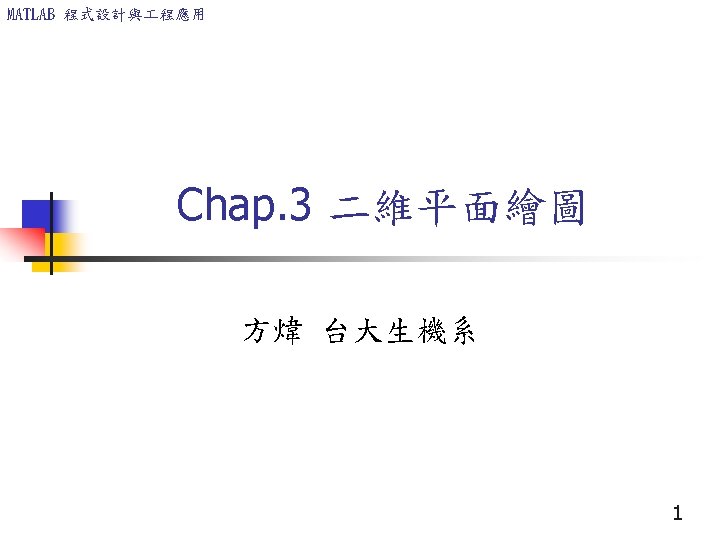
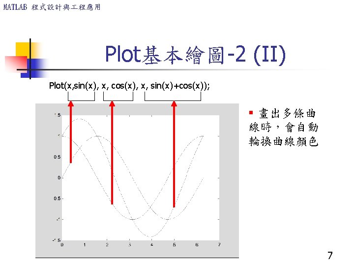
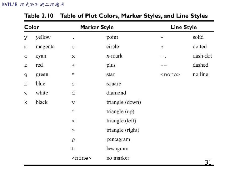
MATLAB 程式設計與 程應用 Z=0. 1+0. 9 i; N=[0: 0. 1: 10]; Plot(z. ^n), xlabel(‘Real’), ylabel(‘Imaginary’); 17
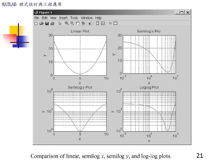

MATLAB 程式設計與 程應用 Ex 4_5. m n n n n n x=0: . 1: 8; y=exp(x); semilogx(x, y); title('Semilogx for y=exp(x)') pause semilogy(x, y); title('Semilogy for y=exp(x)') pause loglog(x, y); title('Loglog for y=exp(x)') 22
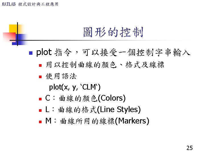


MATLAB 程式設計與 程應用 Enhanced control of plotted lines n Plot(x, y, ’Property. Name’, value, . . ) n Property 的名稱 n n n Line. Width Marker. Edge. Color Marker. Face. Color Marker. Size … X=0: pi/15: 4*pi; y=exp(2*sin(x)); Plot(x, y, ’-ko’, ’Line. Width’, 3, ’Marker. Size’, 6, … ‘Marker. Edge. Color’, ’r’, ‘Marker. Face. Color’, ’g’) 32
. /x; plot(x,")
MATLAB 程式設計與 程應用 Ex 4_7. m close all; x=. 01: 20; y=cos(x). /x; plot(x, y); axis([0 25 -5 5]); %xlim([0, 20]); %ylim([-5, 5]); 36
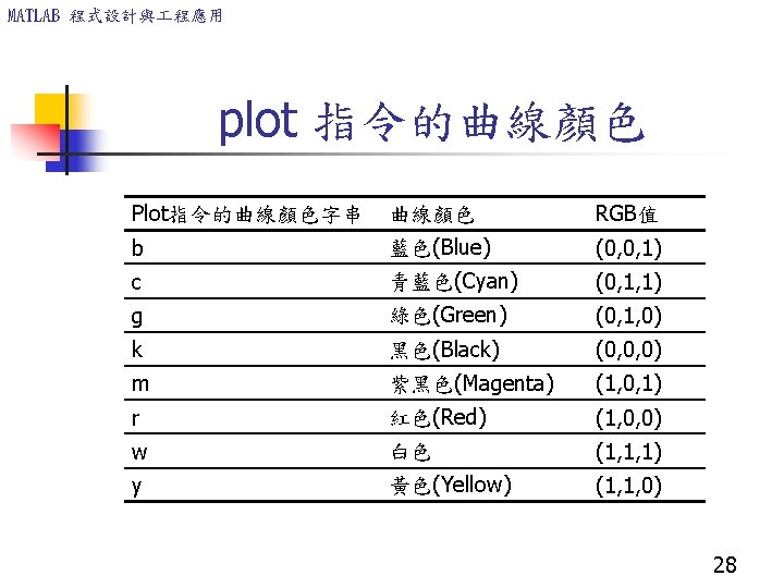
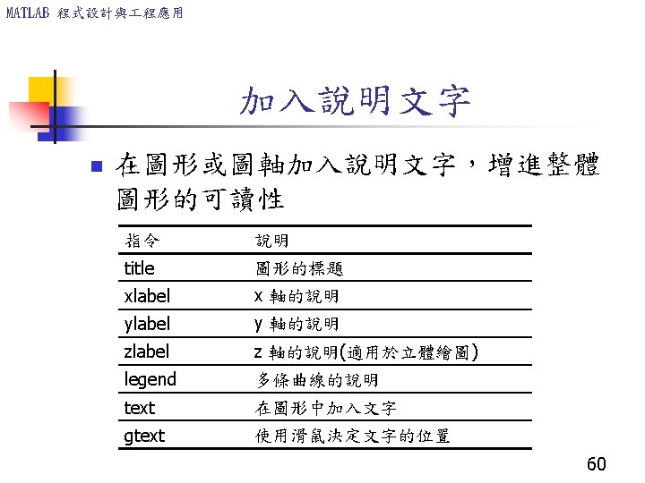
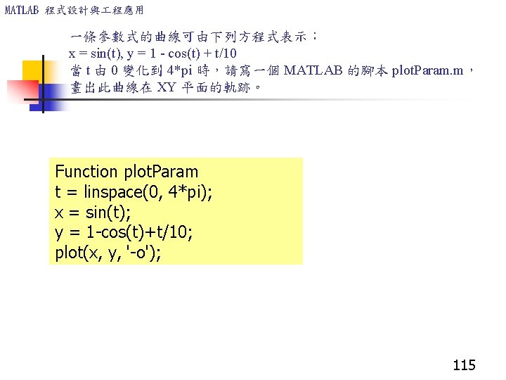
![MATLAB 程式設計與 程應用 圖軸控制範例-4 (I) n 將格線點xtick的數字改為文字 n 範例: x = [1: 6]; y=[13,](http://slidetodoc.com/presentation_image/5995f4392edc9fef2052c101b58d3490/image-41.jpg "MATLAB 程式設計與 程應用 圖軸控制範例-4 (I) n 將格線點xtick的數字改為文字 n 範例: x = [1: 6]; y=[13,")
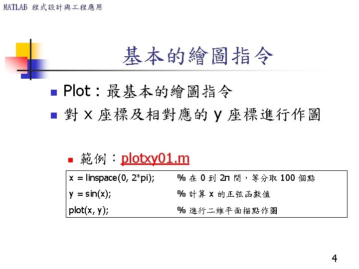
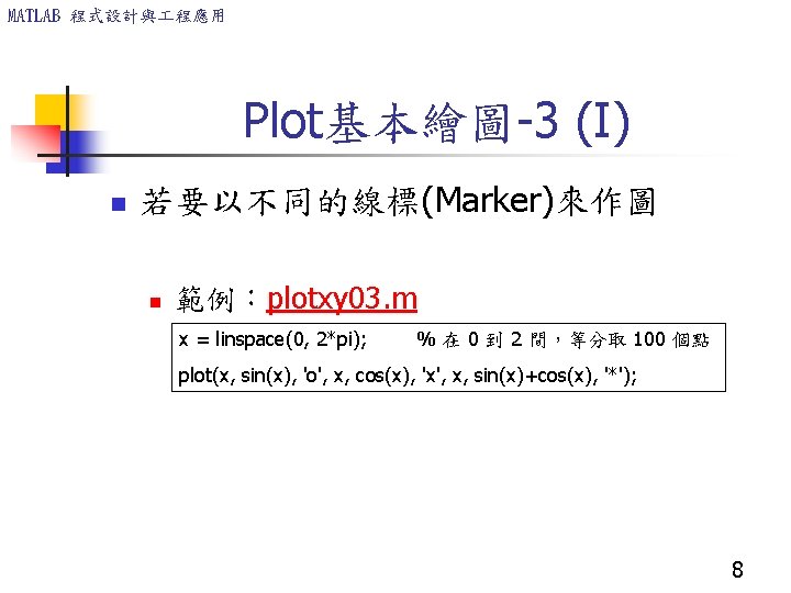
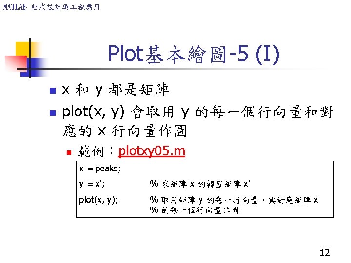
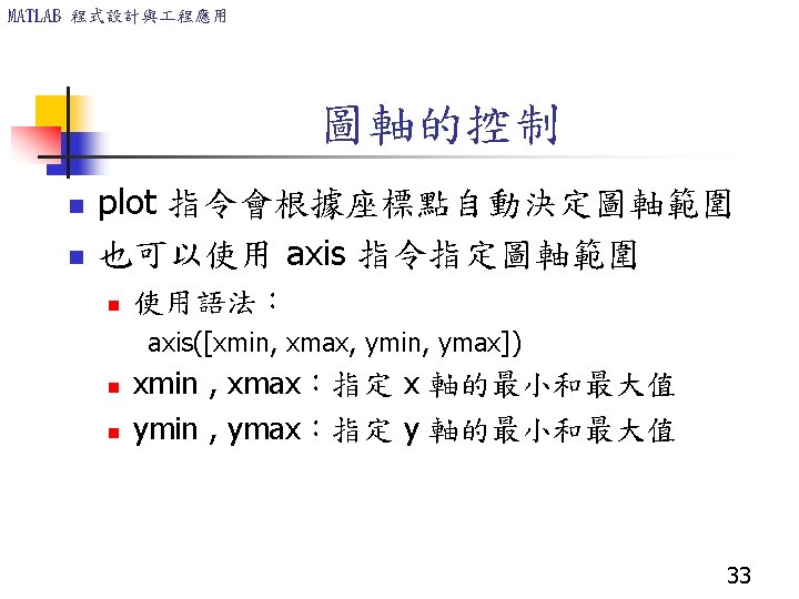
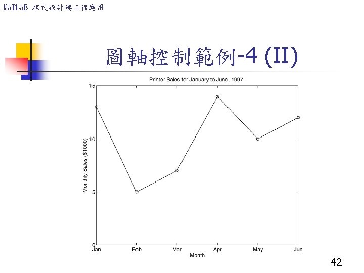
MATLAB 程式設計與 程應用 圖軸控制範例-4 (I) n 將格線點xtick的數字改為文字 n 範例: x = [1: 6]; y=[13, 5, 7, 14, 10, 12]; plot(x, y, ‘o’, x, y) set(gca, ‘xtick', [1: 6], axis([1 6 0 15]), xlabe; (‘Month’); set(gca, ‘xticklabel’, [‘Jan’; ’’Feb’; ’Mar’; ’Apr’; ’May’; ’Jun’]); Ylabel(‘Monthly Sales ($1000)’); Title(‘Printer sales for January to June, 1997’); 41

MATLAB 程式設計與 程應用 一次畫出多條曲線在同一圖上 Ex 4_3. m n n n dx=. 01; x=. 5*dx: 10 -0. 5*dx; y=sin(5*x); y 2=cos(x); % the second function % plot both plot(x, y, 'r-', x, y 2, 'b-'); 43
; y 2=cos(x); plot(x, y 1,")
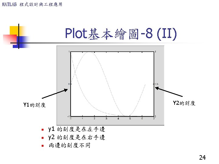
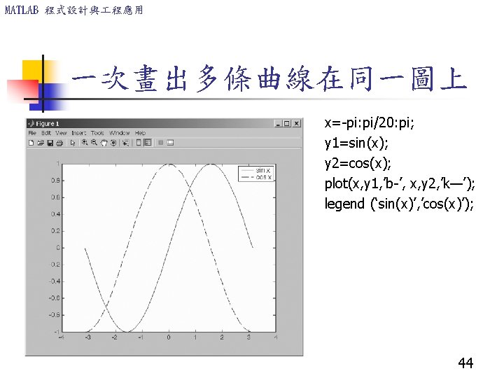
MATLAB 程式設計與 程應用 分批畫出多條曲線在同一圖上 x=-pi: pi/20: pi; y 1=sin(x); y 2=cos(x); plot(x, y 1, ’b-’); hold on; plot(x, y 2, ’k—’); hold off legend (‘sin(x)’, ’cos(x)’); 45
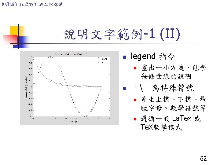
![MATLAB 程式設計與 程應用 legend 指令 x = [0: 0. 01: 2]; y = sinh(x);](http://slidetodoc.com/presentation_image/5995f4392edc9fef2052c101b58d3490/image-46.jpg "MATLAB 程式設計與 程應用 legend 指令 x = [0: 0. 01: 2]; y = sinh(x);")
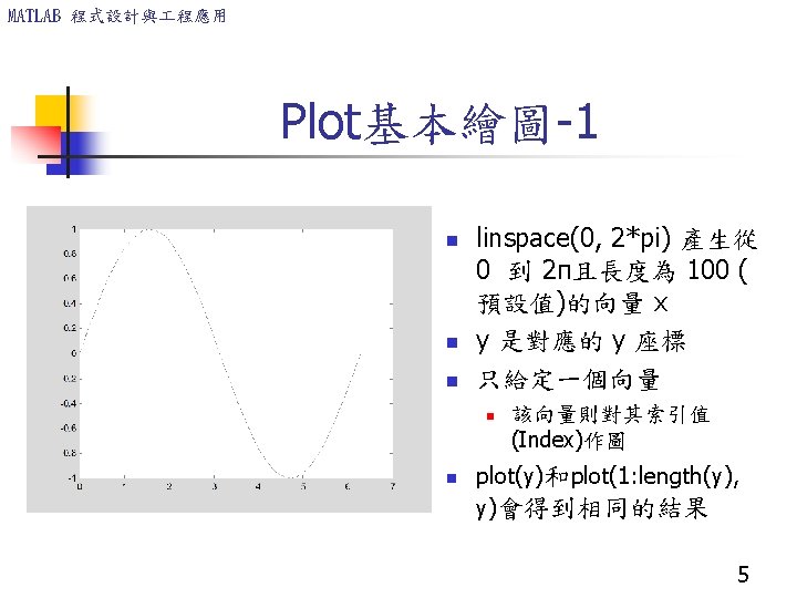
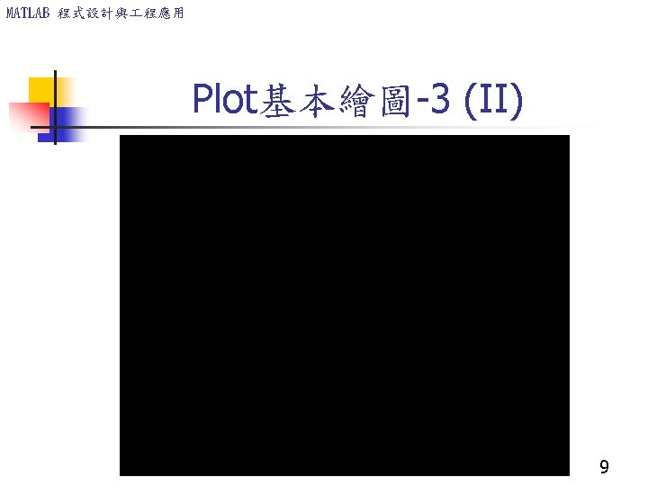
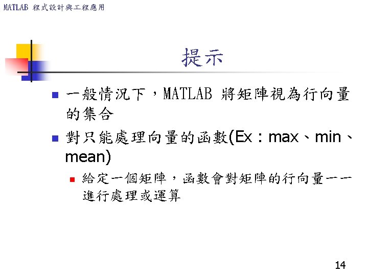
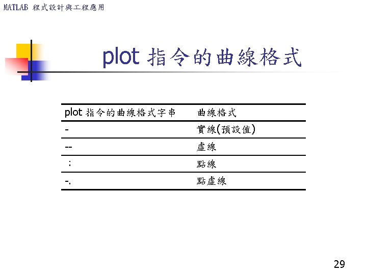
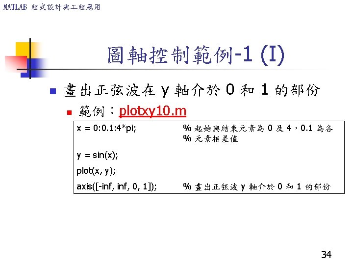
MATLAB 程式設計與 程應用 legend 指令 x = [0: 0. 01: 2]; y = sinh(x); z = tanh(x); plot(x, y, x, z, ’--’), xlabel(’x’), . . . ylabel(’Hyperbolic Sine and Tangent’), . . . legend(’sinh(x)’, ’tanh(x)’) 46

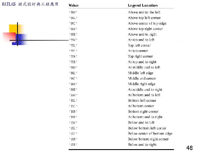
MATLAB 程式設計與 程應用 Possible locations for a plot legend 47
 x=-pi: pi/20: pi; y 1=sin(x); y 2=cos(x); plot(x, y")
MATLAB 程式設計與 程應用 分批畫出多條曲線在不同視窗 figure(1) x=-pi: pi/20: pi; y 1=sin(x); y 2=cos(x); plot(x, y 1, ’b-’); legend (‘sin(x)’); figure(2) plot(x, y 2, ’k—’); legend (’cos(x)’); 49
 Subplot(2, 2, 1 ) Subplot(2, 2, 3 ) Subplot(2,")
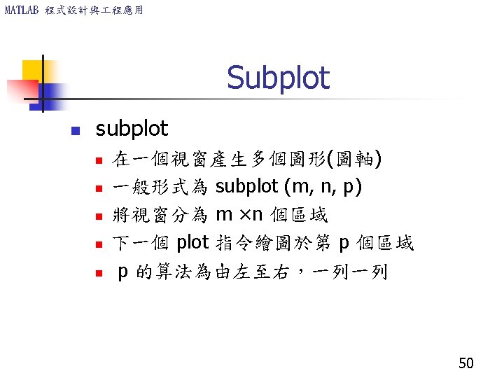
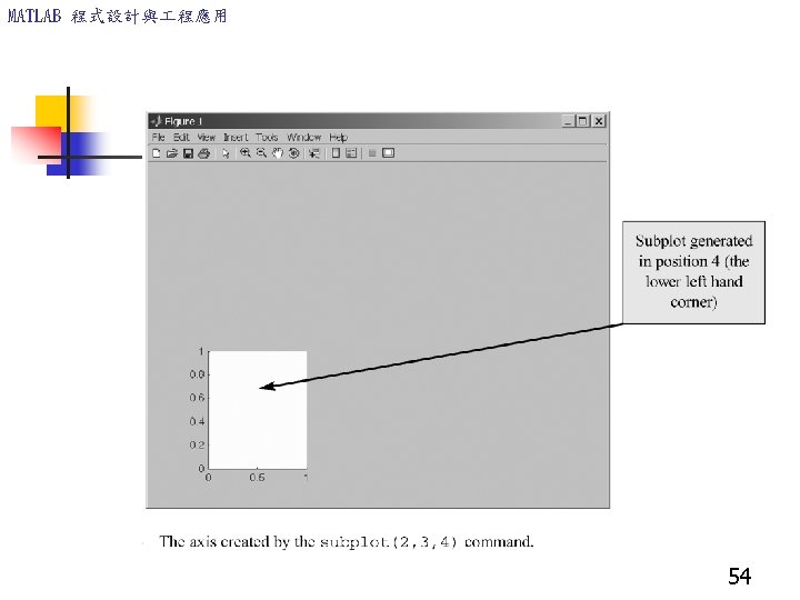
MATLAB 程式設計與 程應用 圖軸控制範例-4 (II) Subplot(2, 2, 1 ) Subplot(2, 2, 3 ) Subplot(2, 2, 2 ) Subplot(2, 2, 4 ) 52
 Subplot(2, 1, 2 ) 53")
MATLAB 程式設計與 程應用 Subplot(2, 1, 1 ) Subplot(2, 1, 2 ) 53
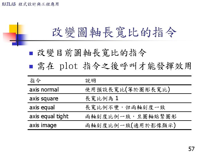
 n 長寬比(Aspect Ratio) n n n 一般圖軸長寬比是視窗的長寬比 可在 axis")
MATLAB 程式設計與 程應用 圖軸控制範例-5 (I) n 長寬比(Aspect Ratio) n n n 一般圖軸長寬比是視窗的長寬比 可在 axis 指令後加不同的字串來修改 範例:plotxy 14. m t = 0: 0. 1: 2*pi; x = 3*cos(t); y = sin(t); subplot(2, 2, 1); plot(x, y); axis normal subplot(2, 2, 2); plot(x, y); axis square subplot(2, 2, 3); plot(x, y); axis equal subplot(2, 2, 4); plot(x, y); axis equal tight 55
 axis normal axis equal axis square axis equal tight")
MATLAB 程式設計與 程應用 圖軸控制範例-5 (II) axis normal axis equal axis square axis equal tight 56
 n 範例:plotxy 15. m subplot(1, 1, 1); x =")
MATLAB 程式設計與 程應用 說明文字範例-1 (I) n 範例:plotxy 15. m subplot(1, 1, 1); x = 0: 0. 1: 2*pi; y 1 = sin(x); y 2 = exp(-x); plot(x, y 1, '--*', x, y 2, ': o'); xlabel('t = 0 to 2pi'); ylabel('values of sin(t) and e^{-x}') title('Function Plots of sin(t) and e^{-x}'); legend('sin(t)', 'e^{-x}'); 61
 n text指令 n n 使用語法: text(x, y, string) x、y")
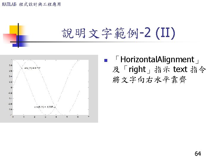
MATLAB 程式設計與 程應用 說明文字範例-2 (I) n text指令 n n 使用語法: text(x, y, string) x、y :文字的起始座標位置 string :代表此文字 範例:plotxy 16. m x = 0: 0. 1: 2*pi; plot(x, sin(x), x, cos(x)); text(pi/4, sin(pi/4), 'leftarrow sin(pi/4) = 0. 707'); text(5*pi/4, cos(5*pi/4), 'cos(5pi/4) = -0. 707rightarrow', 'Horizontal. Alignment', 'right'); 63

MATLAB 程式設計與 程應用 Enhanced control of Text Strings bf Boldface 粗體字 it Italics 斜體字 rm Remove modifiers 取消字體修飾,恢復預設字體 fontname{fontname) 定義使用的字型名稱 fontsize{fontsize} 定義使用的字型大小 _{xxx} {}內的字為下標 ^{xxx} {}內的字為上標 65
")
MATLAB 程式設計與 程應用 練習 ‘bf{B}_{it. S}’ Bs ‘tauit_{m}’ m ‘bfitx_{1}^{2} + x_{2}^{2} rm(units: bfm^{2}rm) ’ 66

MATLAB 程式設計與 程應用 Enhanced control of Text Strings circ sim infty pm leq geq neq prop div int cong leftarrow rightarrow uparrow downarrow leftrightarrow 67
. /x; plot(x,")
MATLAB 程式設計與 程應用 範例:ex 4_1. m close all; x=. 01: 20; y=cos(x). /x; plot(x, y); axis([0 25 -5 5]); str 1='alpha beta gamma delta epsilon phi '; str 2='theta kappa lambda mu nu pi '; str 3='rho sigma tau xi zeta'; xlabel([str 1 str 2 str 3]); text(10, 1, 'theta_1'); text(10, 2, 'theta_{12}'); text(10, 3, 'theta^{10}'); 68
;")
MATLAB 程式設計與 程應用 Ex 4_2. m dx=. 01; x=. 5*dx: 10 -0. 5*dx; y=sin(5*x); %plot(x, y, 'r-'); nhalf=ceil(length(x)/2); plot(x(1: nhalf), y(1: nhalf), 'b-') hold on plot(x(nhalf: end), y(nhalf: end), 'k-') xlabel('theta') ylabel('F(theta)') %title('F(theta)=sin(5 theta)') s=sprintf('F(\theta)=sin(%i \theta)', 5); title(s) 69

MATLAB 程式設計與 程應用 Enhanced control of Text Strings alpha beta lambda mu gamma delta epsilon eta theta tau omega nu pi phi rho sigma Omega Sigma Pi Lambda Delta Gamma 72

MATLAB 程式設計與 程應用 練習:ideal gas law PV=n. RT n n n n n=1; R=8. 314; T=273; P=1: 0. 1: 1000; V=(n*R*T). /P; figure(1); loglog(……); … grid on; hold on; T=373; V=(n*R*T). /P; figure(1); loglog(…); hold off; legend(‘T=273 K’, ’T=373 K’); 請完成本程式,結果如下圖所示 73

MATLAB 程式設計與 程應用 The power function y = 2 x -0. 5 and the exponential function y = 101 -x. 74
 75")
MATLAB 程式設計與 程應用 Exponential function : polyfit(x, y, n) 75
mx. In this case log 10")
MATLAB 程式設計與 程應用 The exponential function: y = b(10)mx. In this case log 10 y = mx + log 10 b which has the form w = p 1 z + p 2 where the polynomial variables w and z are related to the original data variables x and y by w = log 10 y and z = x. We can find the exponential function that fits the data by typing p = polyfit(x, log 10(y), 1) The first element p 1 of the vector p will be m, and the second element p 2 will be log 10 b. We can find b from b = 10 p 2. 76

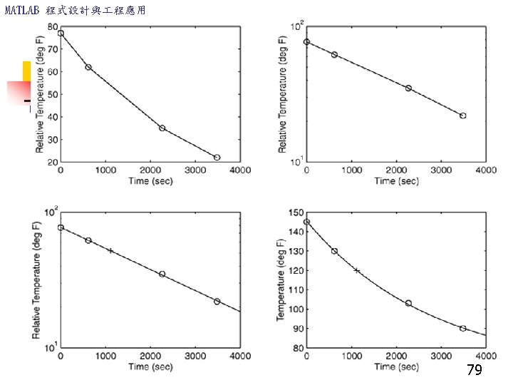
MATLAB 程式設計與 程應用 時間,秒 溫度,o. F 0 145 620 130 2266 103 3482 90 詳見 coffee. m 範例:咖啡冷卻問題 n 室溫 68 o. F下瓷杯內的咖啡由 145 o. F逐漸冷卻,溫度對應於 經過時間的數據如上,請建立溫度對時間的函數,並與 此模式預測,經過多少時間,杯內溫度會達 120 o. F? time=[0, 620, 2266, 3482]; temp=[145, 130, 103, 90]; temp=temp-68; subplot(2, 2, 1); plot(time, temp, ’o’), xlabel(‘Time (sec)’), … ylabel(‘Relative Temperature (deg F)’) subplot(2, 2, 2); semilogy(time, temp, ’o’), xlabel(‘Time (sec)’), … ylabel(‘Relative Temperature (deg F)’) 77
 P=polyfit(time, log 10(temp), 1); m=p(1); b=10^p(2); t_120=(log 10(120 -68)-log")
MATLAB 程式設計與 程應用 範例:咖啡冷卻問題 (續) P=polyfit(time, log 10(temp), 1); m=p(1); b=10^p(2); t_120=(log 10(120 -68)-log 10(b))/m %show thederived curve and estimated point t=[0: 10: 4000]; T=68+b*10. ^(m*t); subplot(2, 2, 3); semilogy(t, T-68, time, temp, 'o', t_120, 120 -68, '+'), xlabel('Time (sec)'), . . . ylabel('Relative Temperature (deg F)'); %show in rectilinear scales subplot(2, 2, 4); plot(t, T, time, temp+68, 'o', t_120, '+'), xlabel('Time (sec)'), . . . ylabel('Temperature (deg F)'); ); 78
 80")
MATLAB 程式設計與 程應用 Power function: polyfit(x, y, n) 80

MATLAB 程式設計與 程應用 The power function: y = bxm. In this case log 10 y = m log 10 x + log 10 b which has the form w = p 1 z + p 2 where the polynomial variables w and z are related to the original data variables x and y by w = log 10 y and z = log 10 x. Thus we can find the power function that fits the data by typing p = polyfit(log 10(x), log 10(y), 1) The first element p 1 of the vector p will be m, and the second element p 2 will be log 10 b. We can find b from b = 10 p 2. 81

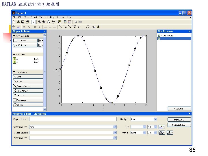
MATLAB 程式設計與 程應用 互動式繪圖 Interactive Plotting 82

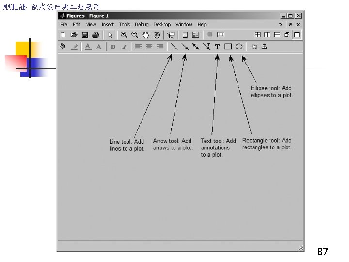
MATLAB 程式設計與 程應用 Tools on the figure toolbar 83

MATLAB 程式設計與 程應用 Edit tool 84


MATLAB 程式設計與 程應用 Figures 的輸出 To save the figure in a format that can be used by another application, such as the standard graphics file formats TIFF or EPS, perform these steps. 1. Select Export Setup from the File menu. This dialog lets you specify options for the output file, such as the figure size, fonts, line size and style, and output format. 2. Select Export from the Export Setup dialog. A standard Save As dialog appears. 3. Select the format from the list of formats in the Save As type menu. This selects the format of the exported file and adds the standard file name extension given to files of that type. 4. Enter the name you want to give the file, less the extension. Then click Save. 91

MATLAB 程式設計與 程應用 Figures 的剪貼 On Windows systems, you can also copy a figure to the clipboard and then paste it into another application: 1. Select Copy Options from the Edit menu. The Copying Options page of the Preferences dialog box appears. 2. Complete the fields on the Copying Options page and click OK. 3. Select Copy Figure from the Edit menu. 92
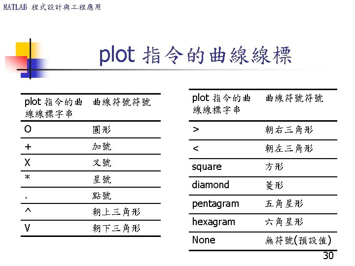
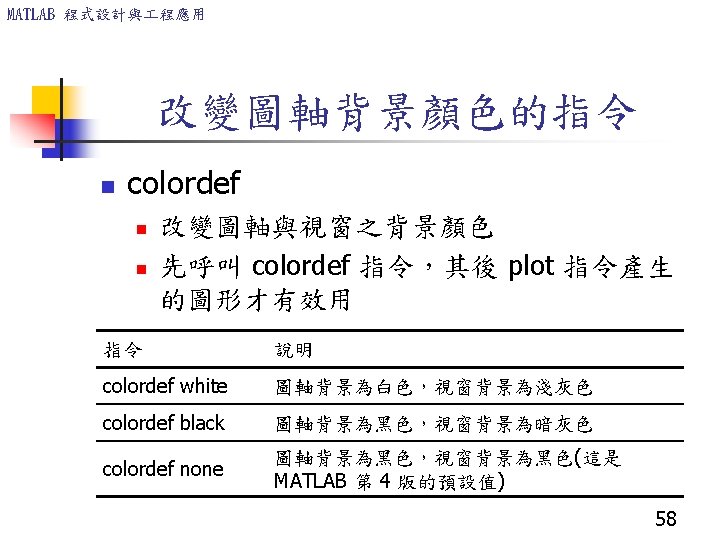
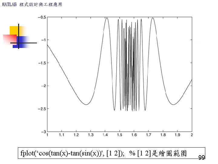
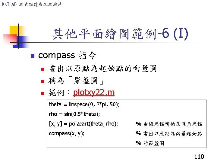
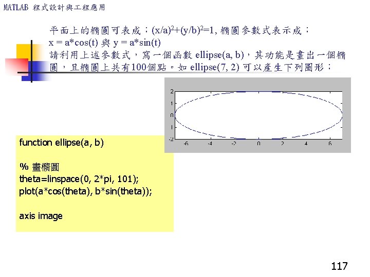
![MATLAB 程式設計與 程應用 x=([1: 0. 01: 2]; plot(x, cos(tan(x)-tan(sin(x))); 98](http://slidetodoc.com/presentation_image/5995f4392edc9fef2052c101b58d3490/image-98.jpg "MATLAB 程式設計與 程應用 x=([1: 0. 01: 2]; plot(x, cos(tan(x)-tan(sin(x))); 98")
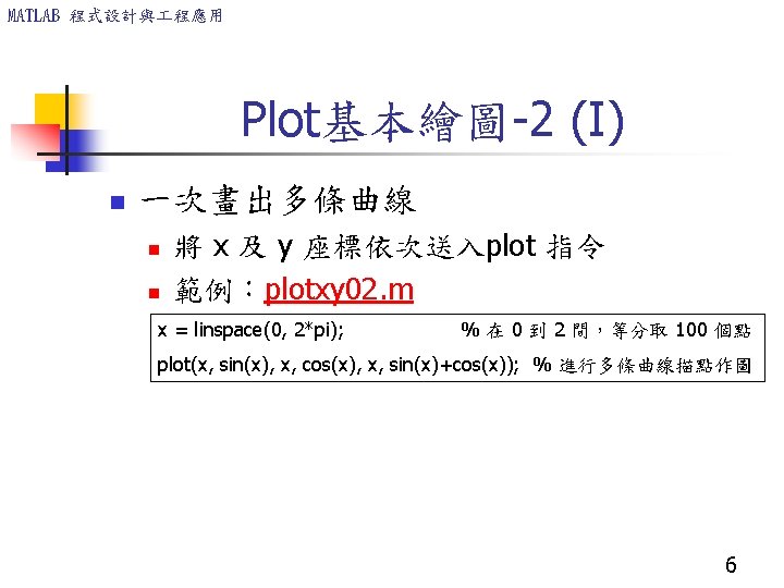
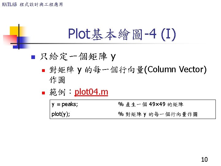
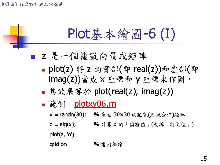
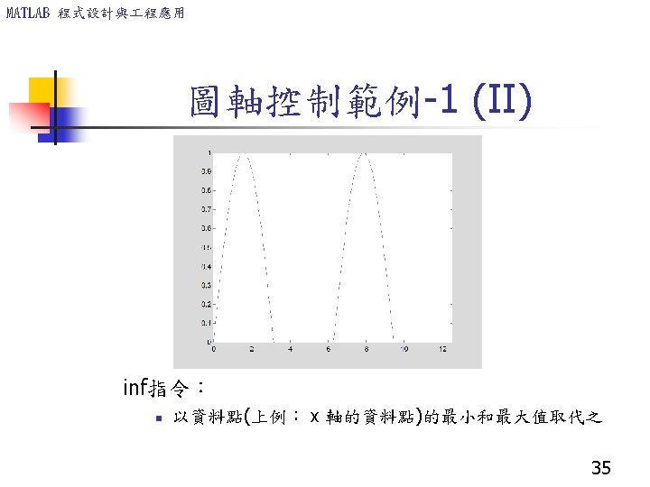
MATLAB 程式設計與 程應用 x=([1: 0. 01: 2]; plot(x, cos(tan(x)-tan(sin(x))); 98

MATLAB 程式設計與 程應用 Plotting Polynomials with the polyval Function. To plot the polynomial 3 x 5 + 2 x 4 – 100 x 3 + 2 x 2 – 7 x + 90 over the range – 6 £ x £ 6 with a spacing of 0. 01, you type >>x = [-6: 0. 01: 6]; >>p = [3, 2, -100, 2, -7, 90]; >>plot(x, polyval(p, x)); >>xlabel(’x’); >>ylabel(’p’); 100
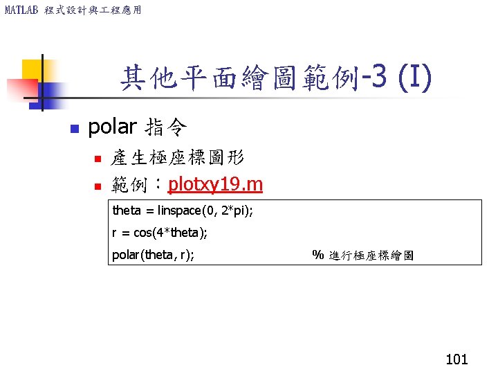


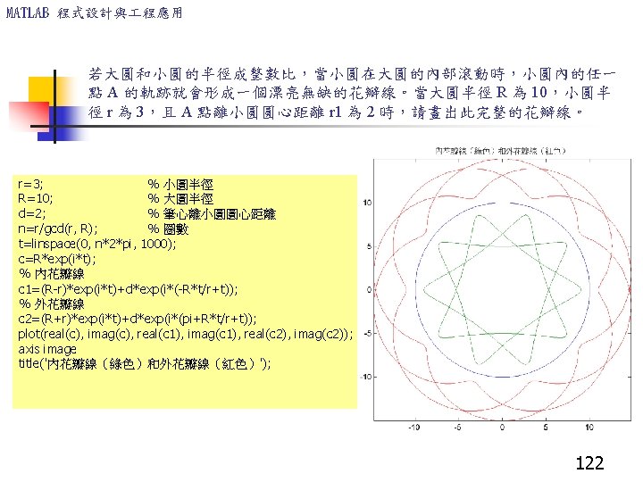
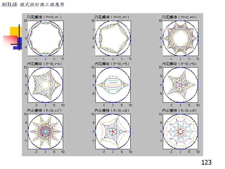
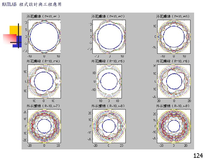
,其功能為畫出一個圓心在 (0, 0)、半 徑為 1 的圓,並在圓內畫出一個內接正 n 邊形,其中一頂點")
MATLAB 程式設計與 程應用 練習 試寫一函數 reg. Poly(n),其功能為畫出一個圓心在 (0, 0)、半 徑為 1 的圓,並在圓內畫出一個內接正 n 邊形,其中一頂點 位於 (0, 1)。例如 reg. Poly(8) 可以畫出如下之正八邊型: function regpoly(n) vertices=[1]; for i=1: n step=2*pi/n; vertices=[vertices, exp(i*step*sqrt(-1))]; end plot(vertices, '-o'); axis image % 畫外接圓 hold on theta=linspace(0, 2*pi); plot(cos(theta), sin(theta), '-r'); hold off axis image 114
,其功能為畫出一個圓心在 (0, 0)、半徑為 1 的 圓,並在圓內畫出一個內接正 n 星形,其中一頂點位於 (0,")
MATLAB 程式設計與 程應用 試寫一函數 reg. Star(n),其功能為畫出一個圓心在 (0, 0)、半徑為 1 的 圓,並在圓內畫出一個內接正 n 星形,其中一頂點位於 (0, 1)。例如 reg. Star(7) 可以畫出如下之正 7 星型: function reg. Star(n) vertices=[1]; for i=1: n step=2*pi*floor(n/2)/n; vertices=[vertices, exp(i*step*sqrt(-1))]; end plot(vertices, '-o'); % 畫外接圓 hold on theta=linspace(0, 2*pi); plot(cos(theta), sin(theta), '-r'); hold off axis image 116
- Slides: 126