1 Overview and Descriptive Statistics Copyright Cengage Learning

1 Overview and Descriptive Statistics Copyright © Cengage Learning. All rights reserved.

1. 3 Measures of Location Copyright © Cengage Learning. All rights reserved.

Measures of Location Visual summaries of data are excellent tools for obtaining preliminary impressions and insights. More formal data analysis often requires the calculation and interpretation of numerical summary measures. That is, from the data we try to extract several summarizing numbers—numbers that might serve to characterize the data set and convey some of its salient features. Our primary concern will be with numerical data; some comments regarding categorical data appear at the end of the section. 3

Measures of Location Suppose, then, that our data set is of the form x 1, x 2, . . . , xn, where each xi is a number. What features of such a set of numbers are of most interest and deserve emphasis? One important characteristic of a set of numbers is its location, and in particular its center. This section presents methods for describing the location of a data set. 4

The Mean 5

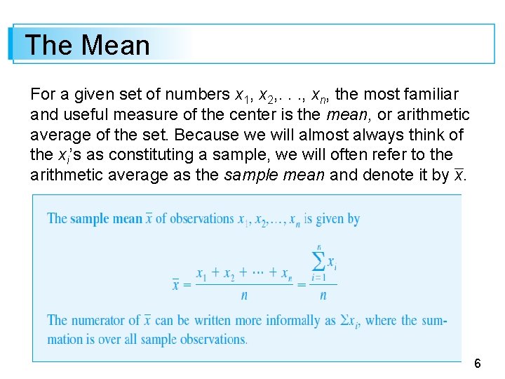
The Mean For a given set of numbers x 1, x 2, . . . , xn, the most familiar and useful measure of the center is the mean, or arithmetic average of the set. Because we will almost always think of the xi’s as constituting a sample, we will often refer to the arithmetic average as the sample mean and denote it by x. 6

The Mean For reporting x, we recommend using decimal accuracy of one digit more than the accuracy of the xi’s. Thus if observations are stopping distances with , x 1 = 125, x 2 = 131, and so on, we might have x = 127. 3 ft. 7

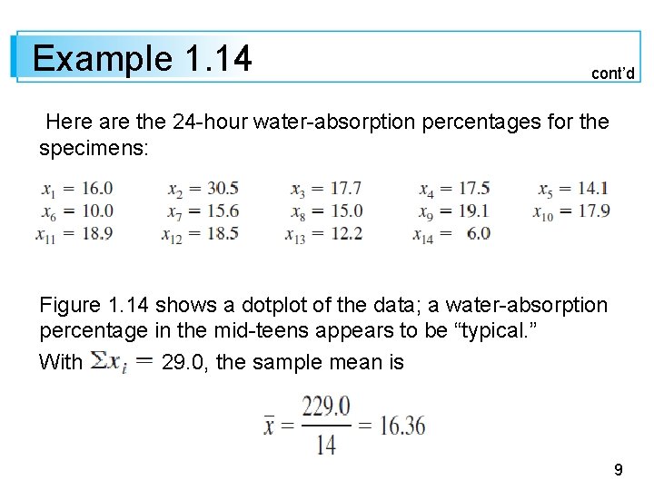
Example 1. 14 Recent years have seen growing commercial interest in the use of what is known as internally cured concrete. This concrete contains porous inclusions most commonly in the form of lightweight aggregate (LWA). The article Characterizing Lightweight Aggregate Desorption at High Relative Humidities Using a Pressure Plate Apparatus” (J. of Materials in Civil Engr, 2012: 961– 969) reported on a study in which researchers examined various physical properties of 14 LWA specimens. 8

Example 1. 14 cont’d Here are the 24 -hour water-absorption percentages for the specimens: Figure 1. 14 shows a dotplot of the data; a water-absorption percentage in the mid-teens appears to be “typical. ” With 229. 0, the sample mean is 9

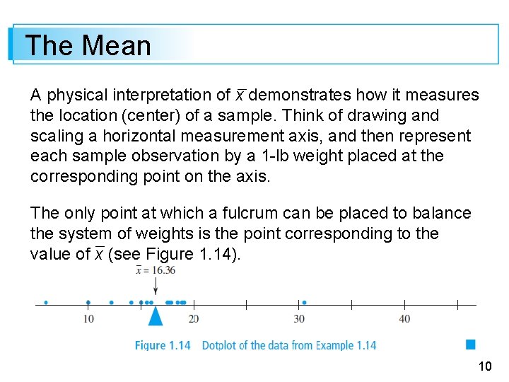
The Mean A physical interpretation of x demonstrates how it measures the location (center) of a sample. Think of drawing and scaling a horizontal measurement axis, and then represent each sample observation by a 1 -lb weight placed at the corresponding point on the axis. The only point at which a fulcrum can be placed to balance the system of weights is the point corresponding to the value of x (see Figure 1. 14). 10

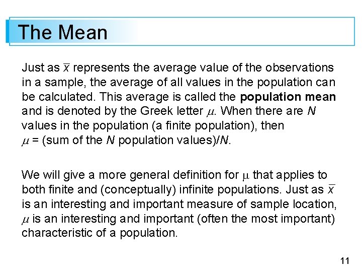
The Mean Just as x represents the average value of the observations in a sample, the average of all values in the population can be calculated. This average is called the population mean and is denoted by the Greek letter . When there are N values in the population (a finite population), then = (sum of the N population values)/N. We will give a more general definition for that applies to both finite and (conceptually) infinite populations. Just as x is an interesting and important measure of sample location, is an interesting and important (often the most important) characteristic of a population. 11

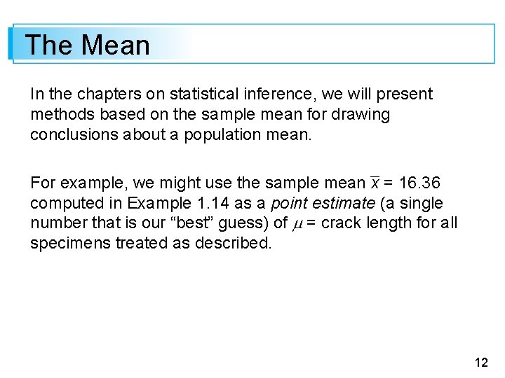
The Mean In the chapters on statistical inference, we will present methods based on the sample mean for drawing conclusions about a population mean. For example, we might use the sample mean x = 16. 36 computed in Example 1. 14 as a point estimate (a single number that is our “best” guess) of = crack length for all specimens treated as described. 12

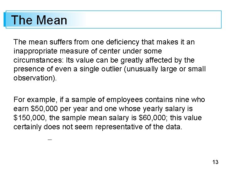
The Mean The mean suffers from one deficiency that makes it an inappropriate measure of center under some circumstances: Its value can be greatly affected by the presence of even a single outlier (unusually large or small observation). For example, if a sample of employees contains nine who earn $50, 000 per year and one whose yearly salary is $150, 000, the sample mean salary is $60, 000; this value certainly does not seem representative of the data. 13

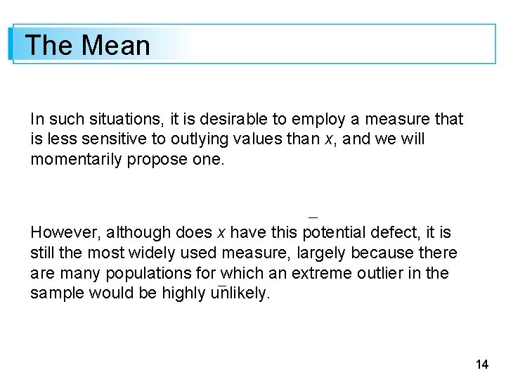
The Mean In such situations, it is desirable to employ a measure that is less sensitive to outlying values than x, and we will momentarily propose one. However, although does x have this potential defect, it is still the most widely used measure, largely because there are many populations for which an extreme outlier in the sample would be highly unlikely. 14

The Mean When sampling from such a population (a normal or bellshaped population being the most important example), the sample mean will tend to be stable and quite representative of the sample. 15

The Median 16

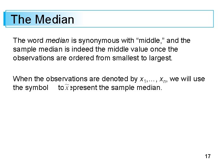
The Median The word median is synonymous with “middle, ” and the sample median is indeed the middle value once the observations are ordered from smallest to largest. When the observations are denoted by x 1, …, xn, we will use the symbol to represent the sample median. 17

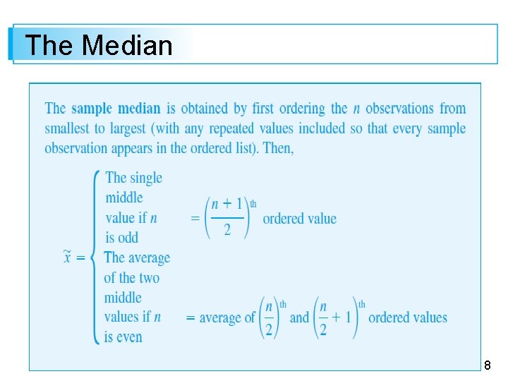
The Median 18

Example 1. 15 People not familiar with classical music might tend to believe that a composer’s instructions for playing a particular piece are so specific that the duration would not depend at all on the performer(s). However, there is typically plenty of room for interpretation, and orchestral conductors and musicians take full advantage of this. 19

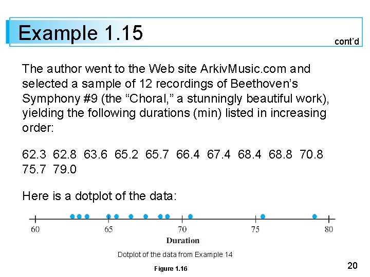
Example 1. 15 cont’d The author went to the Web site Arkiv. Music. com and selected a sample of 12 recordings of Beethoven’s Symphony #9 (the “Choral, ” a stunningly beautiful work), yielding the following durations (min) listed in increasing order: 62. 3 62. 8 63. 6 65. 2 65. 7 66. 4 67. 4 68. 8 70. 8 75. 7 79. 0 Here is a dotplot of the data: Dotplot of the data from Example 14 Figure 1. 16 20

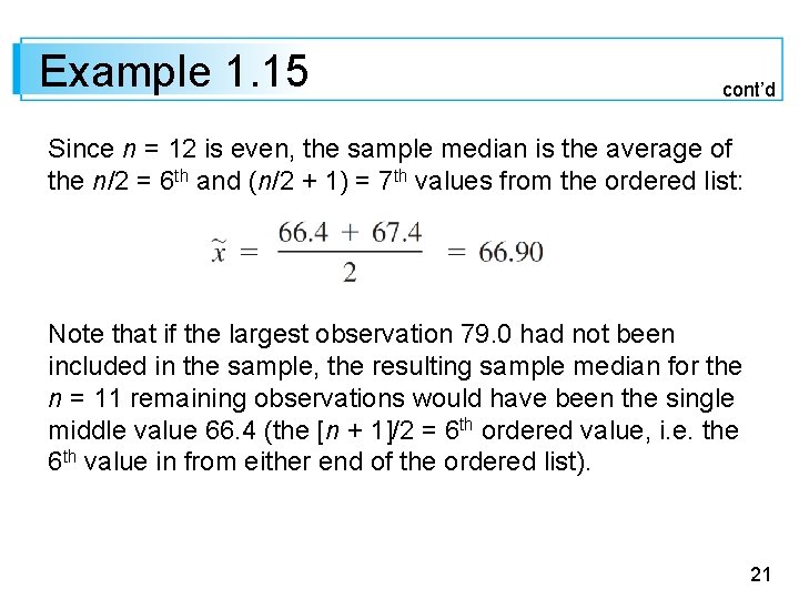
Example 1. 15 cont’d Since n = 12 is even, the sample median is the average of the n/2 = 6 th and (n/2 + 1) = 7 th values from the ordered list: Note that if the largest observation 79. 0 had not been included in the sample, the resulting sample median for the n = 11 remaining observations would have been the single middle value 66. 4 (the [n + 1]/2 = 6 th ordered value, i. e. the 6 th value in from either end of the ordered list). 21

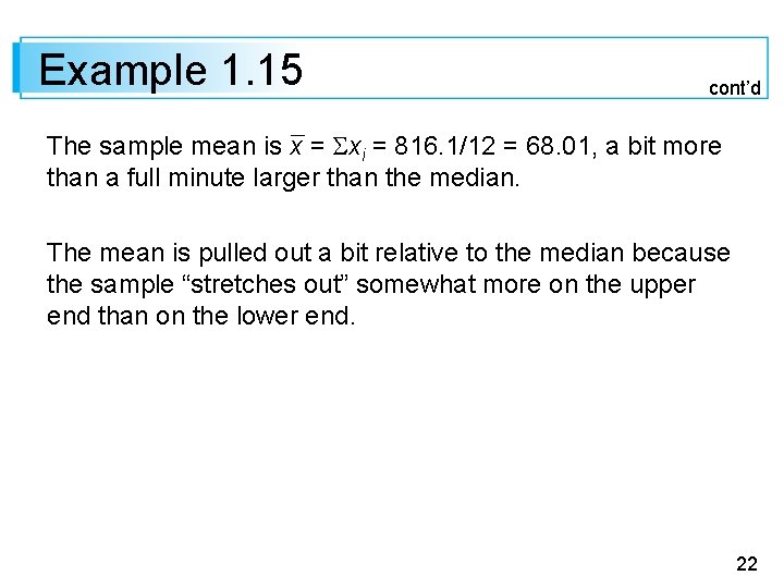
Example 1. 15 cont’d The sample mean is x = xi = 816. 1/12 = 68. 01, a bit more than a full minute larger than the median. The mean is pulled out a bit relative to the median because the sample “stretches out” somewhat more on the upper end than on the lower end. 22

The Median The data in Example 1. 15 illustrates an important property of in contrast to x: The sample median is very insensitive to outliers. If, for example, we increased the two largest xis from 75. 7 and 79. 0 to 85. 7 and 89. 0, respectively, would be unaffected. Thus, in the treatment of outlying data values, x and are at opposite ends of a spectrum. Both quantities describe where the data is centered, but they will not in general be equal because they focus on different aspects of the sample. 23

The Median Analogous to as the middle value in the sample is a middle value in the population, the population median, denoted by As with and , we can think of using the sample median to make an inference about In Example 1. 15, we might use = 66. 90 as an estimate of the median time for the population of all recordings. A median is often used to describe income or salary data (because it is not greatly influenced by a few large salaries). 24

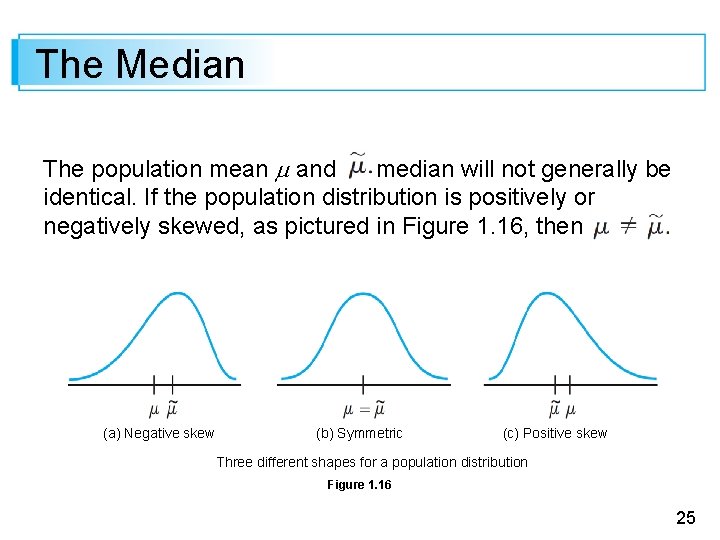
The Median The population mean and median will not generally be identical. If the population distribution is positively or negatively skewed, as pictured in Figure 1. 16, then (a) Negative skew (b) Symmetric (c) Positive skew Three different shapes for a population distribution Figure 1. 16 25

The Median When this is the case, in making inferences we must first decide which of the two population characteristics is of greater interest and then proceed accordingly. 26

Other Measures of Location: Quartiles, Percentiles, and Trimmed Means 27

Other Measures of Location: Quartiles, Percentiles, and Trimmed Means The median (population or sample) divides the data set into two parts of equal size. To obtain finer measures of location, we could divide the data into more than two such parts. Roughly speaking, quartiles divide the data set into four equal parts, with the observations above third quartile constituting the upper quarter of the data set, the second quartile being identical to the median, and the first quartile separating the lower quarter from the upper three-quarters. 28

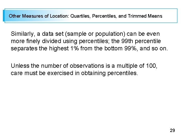
Other Measures of Location: Quartiles, Percentiles, and Trimmed Means Similarly, a data set (sample or population) can be even more finely divided using percentiles; the 99 th percentile separates the highest 1% from the bottom 99%, and so on. Unless the number of observations is a multiple of 100, care must be exercised in obtaining percentiles. 29

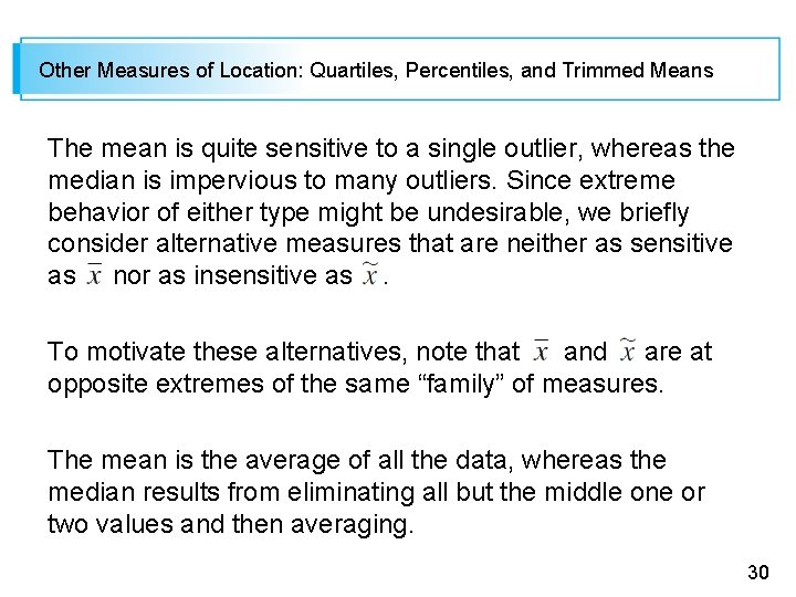
Other Measures of Location: Quartiles, Percentiles, and Trimmed Means The mean is quite sensitive to a single outlier, whereas the median is impervious to many outliers. Since extreme behavior of either type might be undesirable, we briefly consider alternative measures that are neither as sensitive as nor as insensitive as. To motivate these alternatives, note that and are at opposite extremes of the same “family” of measures. The mean is the average of all the data, whereas the median results from eliminating all but the middle one or two values and then averaging. 30

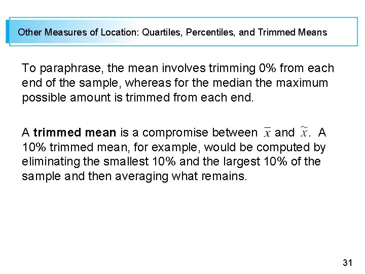
Other Measures of Location: Quartiles, Percentiles, and Trimmed Means To paraphrase, the mean involves trimming 0% from each end of the sample, whereas for the median the maximum possible amount is trimmed from each end. A trimmed mean is a compromise between and. A 10% trimmed mean, for example, would be computed by eliminating the smallest 10% and the largest 10% of the sample and then averaging what remains. 31

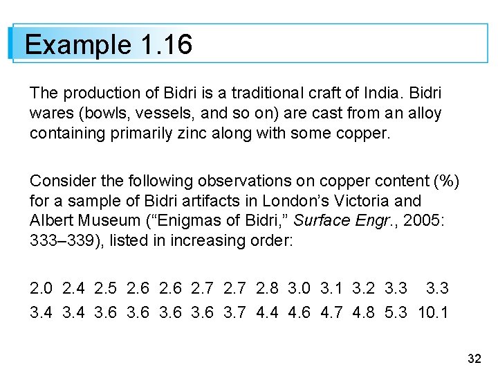
Example 1. 16 The production of Bidri is a traditional craft of India. Bidri wares (bowls, vessels, and so on) are cast from an alloy containing primarily zinc along with some copper. Consider the following observations on copper content (%) for a sample of Bidri artifacts in London’s Victoria and Albert Museum (“Enigmas of Bidri, ” Surface Engr. , 2005: 333– 339), listed in increasing order: 2. 0 2. 4 2. 5 2. 6 2. 7 2. 8 3. 0 3. 1 3. 2 3. 3 3. 4 3. 6 3. 7 4. 4 4. 6 4. 7 4. 8 5. 3 10. 1 32

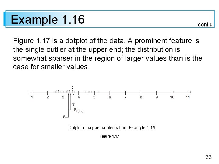
Example 1. 16 cont’d Figure 1. 17 is a dotplot of the data. A prominent feature is the single outlier at the upper end; the distribution is somewhat sparser in the region of larger values than is the case for smaller values. Dotplot of copper contents from Example 1. 16 Figure 1. 17 33

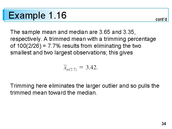
Example 1. 16 cont’d The sample mean and median are 3. 65 and 3. 35, respectively. A trimmed mean with a trimming percentage of 100(2/26) = 7. 7% results from eliminating the two smallest and two largest observations; this gives Trimming here eliminates the larger outlier and so pulls the trimmed mean toward the median. 34

Other Measures of Location: Quartiles, Percentiles, and Trimmed Means A trimmed mean with a moderate trimming percentage—someplace between 5% and 25%—will yield a measure of center that is neither as sensitive to outliers as is the mean nor as insensitive as the median. If the desired trimming percentage is 100 % and n is not an integer, the trimmed mean must be calculated by interpolation. For example, consider =. 10 for a 10% trimming percentage and n = 26 as in Example 1. 16. 35

Other Measures of Location: Quartiles, Percentiles, and Trimmed Means Then xtr(10) would be the appropriate weighted average of the 7. 7% trimmed mean calculated there and the 11. 5% trimmed mean resulting from trimming three observations from each end. 36

Categorical Data and Sample Proportions 37

Categorical Data and Sample Proportions When the data is categorical, a frequency distribution or relative frequency distribution provides an effective tabular summary of the data. The natural numerical summary quantities in this situation are the individual frequencies and the relative frequencies. For example, if a survey of individuals who own digital cameras is undertaken to study brand preference, then each individual in the sample would identify the brand of camera that he or she owned, from which we could count the number owning Canon, Sony, Kodak, and so on. 38

Categorical Data and Sample Proportions Consider sampling a dichotomous population—one that consists of only two categories (such as voted or did not vote in the last election, does or does not own a digital camera, etc. ). If we let x denote the number in the sample falling in category 1, then the number in category 2 is n – x. The relative frequency or sample proportion in category 1 is x/n and the sample proportion in category 2 is 1 – x/n. 39

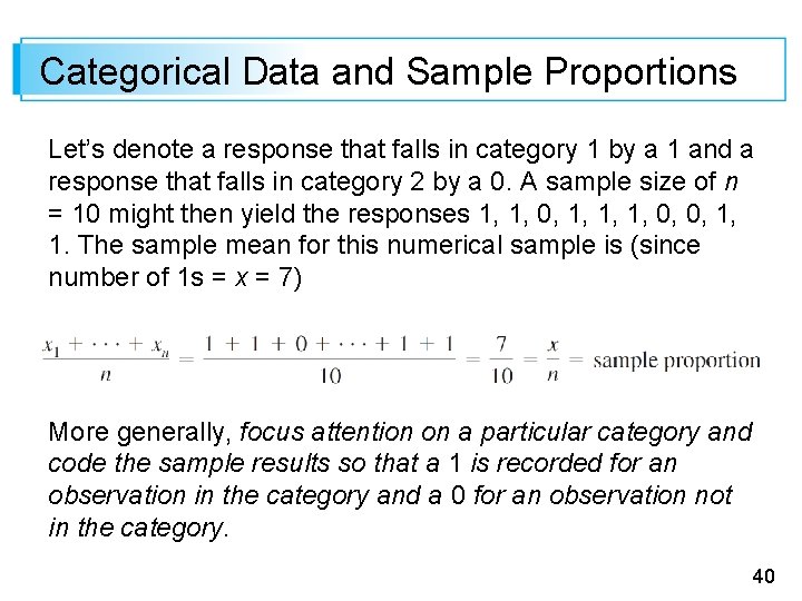
Categorical Data and Sample Proportions Let’s denote a response that falls in category 1 by a 1 and a response that falls in category 2 by a 0. A sample size of n = 10 might then yield the responses 1, 1, 0, 1, 1, 1, 0, 0, 1, 1. The sample mean for this numerical sample is (since number of 1 s = x = 7) More generally, focus attention on a particular category and code the sample results so that a 1 is recorded for an observation in the category and a 0 for an observation not in the category. 40

Categorical Data and Sample Proportions Then the sample proportion of observations in the category is the sample mean of the sequence of 1 s and 0 s. Thus a sample mean can be used to summarize the results of a categorical sample. These remarks also apply to situations in which categories are defined by grouping values in a numerical sample or population (e. g. , we might be interested in knowing whether individuals have owned their present automobile for at least 5 years, rather than studying the exact length of ownership). 41

Categorical Data and Sample Proportions Analogous to the sample proportion x/n of individuals or objects falling in a particular category, let p represent the proportion of those in the entire population falling in the category. As with x/n, p is a quantity between 0 and 1, and while x/n is a sample characteristic, p is a characteristic of the population. 42

Categorical Data and Sample Proportions The relationship between the two parallels the relationship between and between x and . In particular, we will subsequently use x/n to make inferences about p. If a sample of 100 students from a large university reveals that 38 have Macintosh computers, then we could use 38/100 5. 38 as a point estimate of the proportion of all students at the university who have Macs. Or we might ask whether this sample provides strong evidence for concluding that at least 1/3 of all students are Mac owners. 43

Categorical Data and Sample Proportions With k categories (k. 2), we can use the k sample proportions to answer questions about the population proportions p 1, …, pk. 44