1 Overview and Descriptive Statistics Copyright Cengage Learning

1 Overview and Descriptive Statistics Copyright © Cengage Learning. All rights reserved.

1. 4 Measures of Variability Copyright © Cengage Learning. All rights reserved.

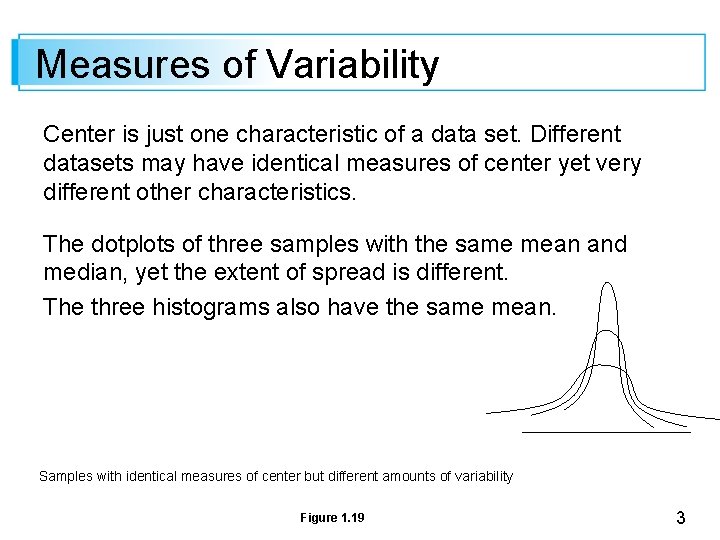
Measures of Variability Center is just one characteristic of a data set. Different datasets may have identical measures of center yet very different other characteristics. The dotplots of three samples with the same mean and median, yet the extent of spread is different. The three histograms also have the same mean. Samples with identical measures of center but different amounts of variability Figure 1. 19 3

Measures of Variability for Sample Data 4

Measures of Variability for Sample Data: Range Simple measure: range, is the difference between the largest and smallest sample values. The range for sample 1 is much larger than sample 3, so it has more variability. A defect: it depends on the two most extreme observations only and disregards the remaining n – 2 values. Samples 1 and 2 have identical ranges, yet there is much less variability or dispersion in the second sample than in the first. 5

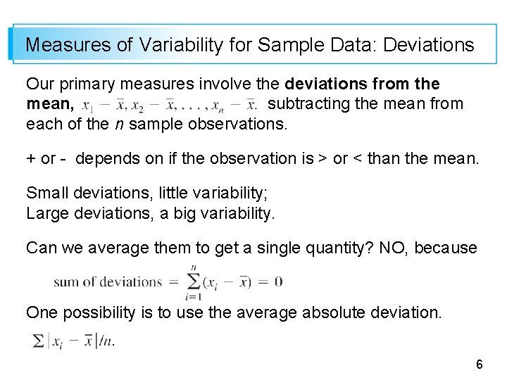
Measures of Variability for Sample Data: Deviations Our primary measures involve the deviations from the mean, , subtracting the mean from each of the n sample observations. + or - depends on if the observation is > or < than the mean. Small deviations, little variability; Large deviations, a big variability. Can we average them to get a single quantity? NO, because One possibility is to use the average absolute deviation. 6

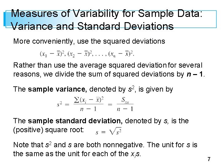
Measures of Variability for Sample Data: Variance and Standard Deviations More conveniently, use the squared deviations Rather than use the average squared deviation for several reasons, we divide the sum of squared deviations by n – 1. The sample variance, denoted by s 2, is given by The sample standard deviation, denoted by s, is the (positive) square root: Note that s 2 and s are both nonnegative. The unit for s is the same as the unit for each of the xis. 7

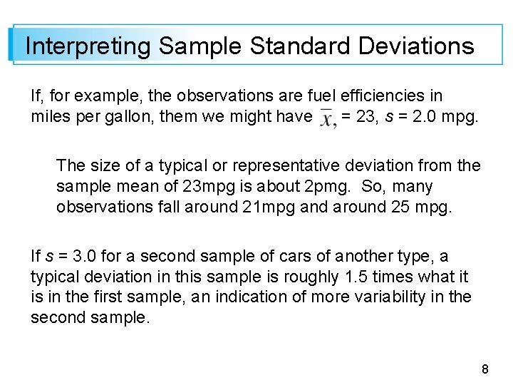
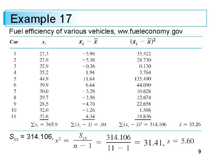
Interpreting Sample Standard Deviations If, for example, the observations are fuel efficiencies in miles per gallon, them we might have = 23, s = 2. 0 mpg. The size of a typical or representative deviation from the sample mean of 23 mpg is about 2 pmg. So, many observations fall around 21 mpg and around 25 mpg. If s = 3. 0 for a second sample of cars of another type, a typical deviation in this sample is roughly 1. 5 times what it is in the first sample, an indication of more variability in the second sample. 8

Example 17 Fuel efficiency of various vehicles, ww. fueleconomy. gov Sxx = 314. 106, , 9

Motivation for s 2 Why divided by n-1 instead of n 10

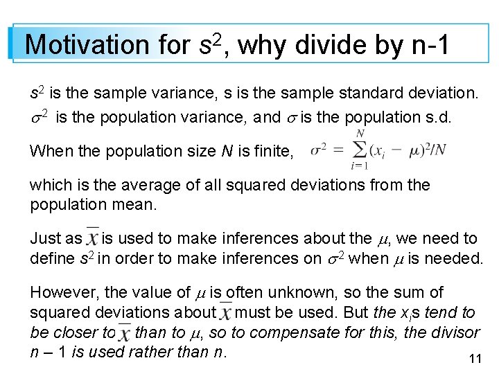
Motivation for s 2, why divide by n-1 s 2 is the sample variance, s is the sample standard deviation. 2 is the population variance, and is the population s. d. When the population size N is finite, which is the average of all squared deviations from the population mean. Just as is used to make inferences about the , we need to define s 2 in order to make inferences on 2 when is needed. However, the value of is often unknown, so the sum of squared deviations about must be used. But the xis tend to be closer to than to , so to compensate for this, the divisor n – 1 is used rather than n. 11

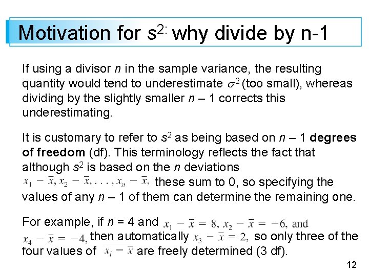
Motivation for s 2: why divide by n-1 If using a divisor n in the sample variance, the resulting quantity would tend to underestimate 2 (too small), whereas dividing by the slightly smaller n – 1 corrects this underestimating. It is customary to refer to s 2 as being based on n – 1 degrees of freedom (df). This terminology reflects the fact that although s 2 is based on the n deviations these sum to 0, so specifying the values of any n – 1 of them can determine the remaining one. For example, if n = 4 and then automatically so only three of the four values of are freely determined (3 df). 12

A Computing Formula for s 2 13

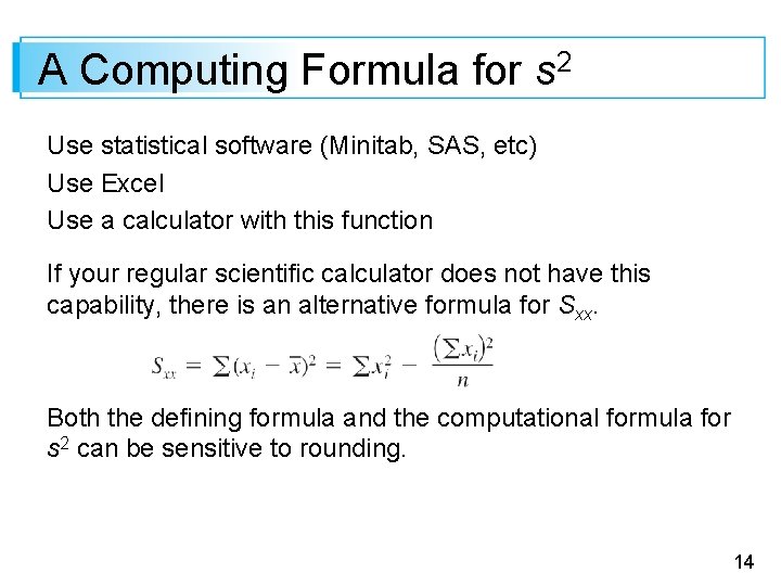
A Computing Formula for s 2 Use statistical software (Minitab, SAS, etc) Use Excel Use a calculator with this function If your regular scientific calculator does not have this capability, there is an alternative formula for Sxx. Both the defining formula and the computational formula for s 2 can be sensitive to rounding. 14

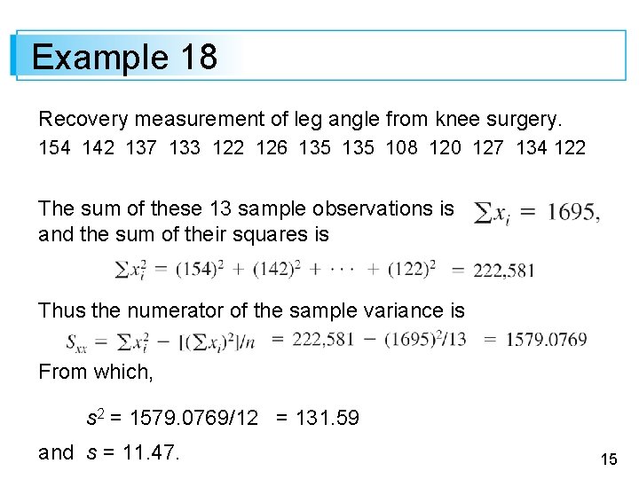
Example 18 Recovery measurement of leg angle from knee surgery. 154 142 137 133 122 126 135 108 120 127 134 122 The sum of these 13 sample observations is and the sum of their squares is Thus the numerator of the sample variance is From which, s 2 = 1579. 0769/12 = 131. 59 and s = 11. 47. 15

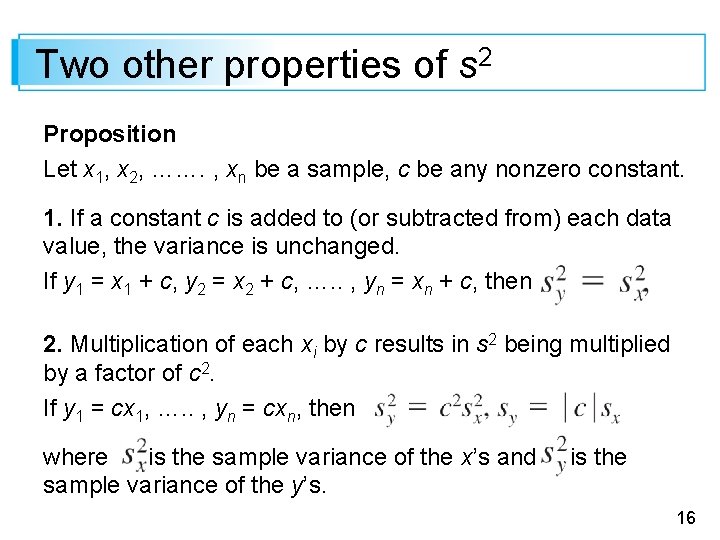
Two other properties of s 2 Proposition Let x 1, x 2, ……. , xn be a sample, c be any nonzero constant. 1. If a constant c is added to (or subtracted from) each data value, the variance is unchanged. If y 1 = x 1 + c, y 2 = x 2 + c, …. . , yn = xn + c, then 2. Multiplication of each xi by c results in s 2 being multiplied by a factor of c 2. If y 1 = cx 1, …. . , yn = cxn, then where is the sample variance of the x’s and sample variance of the y’s. is the 16

Boxplots 17

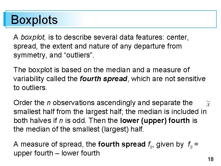
Boxplots A boxplot, is to describe several data features: center, spread, the extent and nature of any departure from symmetry, and “outliers”. The boxplot is based on the median and a measure of variability called the fourth spread, which are not sensitive to outliers. Order the n observations ascendingly and separate the smallest half from the largest half; the median is included in both halves if n is odd. Then the lower (upper) fourth is the median of the smallest (largest) half. A measure of spread, the fourth spread fs, given by fs = upper fourth – lower fourth 18

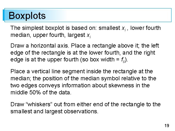
Boxplots The simplest boxplot is based on: smallest xi , lower fourth median, upper fourth, largest xi Draw a horizontal axis. Place a rectangle above it; the left edge of the rectangle is at the lower fourth, and the right edge is at the upper fourth (so box width = fs). Place a vertical line segment inside the rectangle at the median; the position of the median symbol relative to the two edges conveys information about skewness in the middle 50% of the data. Draw “whiskers” out from either end of the rectangle to the smallest and largest observations. 19

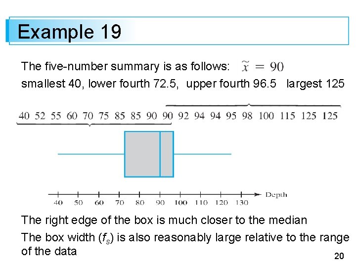
Example 19 The five-number summary is as follows: smallest 40, lower fourth 72. 5, upper fourth 96. 5 largest 125 The right edge of the box is much closer to the median The box width (fs) is also reasonably large relative to the range of the data 20

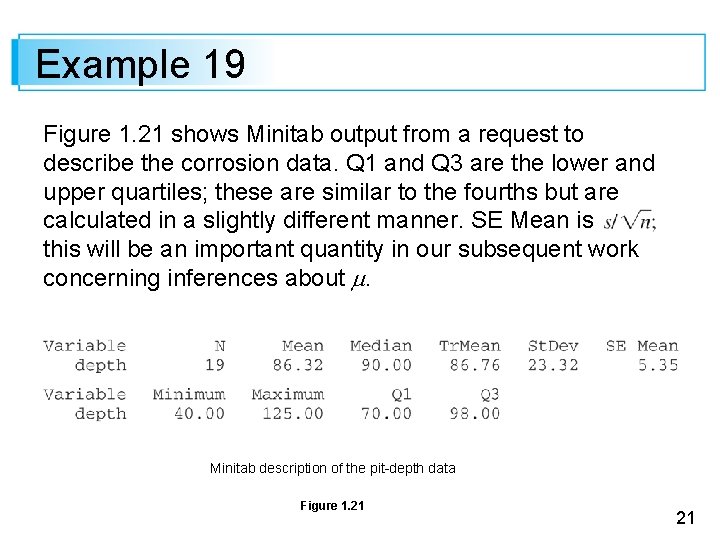
Example 19 Figure 1. 21 shows Minitab output from a request to describe the corrosion data. Q 1 and Q 3 are the lower and upper quartiles; these are similar to the fourths but are calculated in a slightly different manner. SE Mean is this will be an important quantity in our subsequent work concerning inferences about . Minitab description of the pit-depth data Figure 1. 21 21

Boxplots That Show Outliers 22

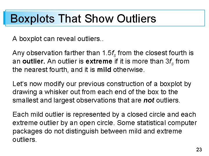
Boxplots That Show Outliers A boxplot can reveal outliers. . Any observation farther than 1. 5 fs from the closest fourth is an outlier. An outlier is extreme if it is more than 3 fs from the nearest fourth, and it is mild otherwise. Let’s now modify our previous construction of a boxplot by drawing a whisker out from each end of the box to the smallest and largest observations that are not outliers. Each mild outlier is represented by a closed circle and each extreme outlier by an open circle. Some statistical computer packages do not distinguish between mild and extreme outliers. 23

Boxplots That Show Outliers Let’s now modify our previous construction of a boxplot by drawing a whisker out from each end of the box to the smallest and largest observations that are not outliers. Each mild outlier is represented by a closed circle and each extreme outlier by an open circle. Some statistical computer packages do not distinguish between mild and extreme outliers. 24

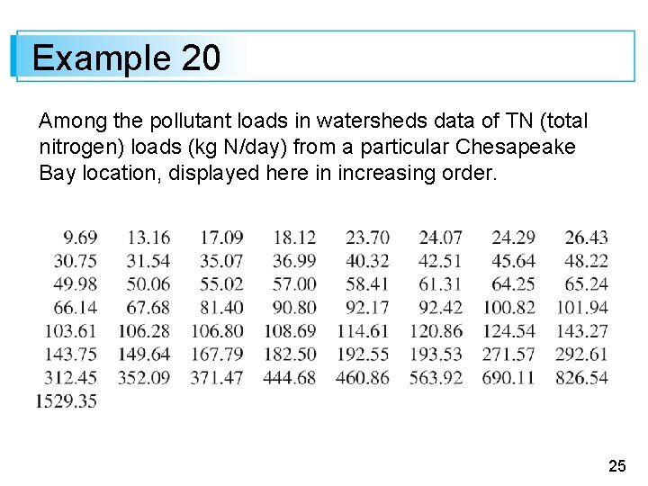
Example 20 Among the pollutant loads in watersheds data of TN (total nitrogen) loads (kg N/day) from a particular Chesapeake Bay location, displayed here in increasing order. 25

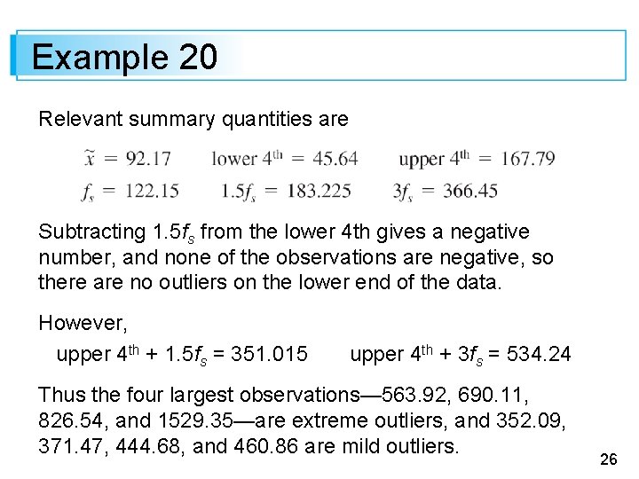
Example 20 Relevant summary quantities are Subtracting 1. 5 fs from the lower 4 th gives a negative number, and none of the observations are negative, so there are no outliers on the lower end of the data. However, upper 4 th + 1. 5 fs = 351. 015 upper 4 th + 3 fs = 534. 24 Thus the four largest observations— 563. 92, 690. 11, 826. 54, and 1529. 35—are extreme outliers, and 352. 09, 371. 47, 444. 68, and 460. 86 are mild outliers. 26

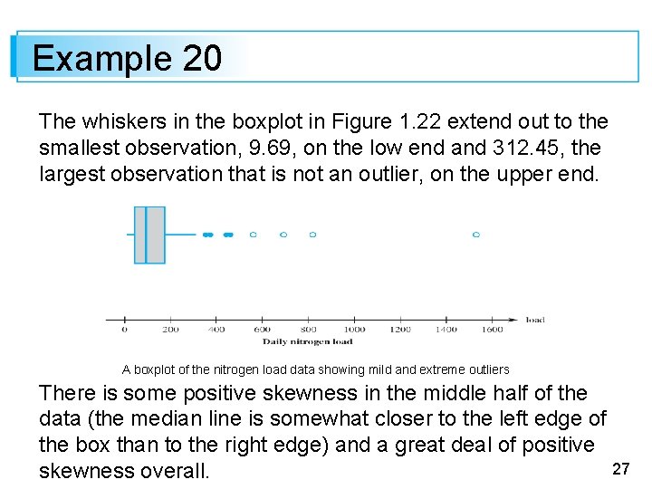
Example 20 The whiskers in the boxplot in Figure 1. 22 extend out to the smallest observation, 9. 69, on the low end and 312. 45, the largest observation that is not an outlier, on the upper end. A boxplot of the nitrogen load data showing mild and extreme outliers There is some positive skewness in the middle half of the data (the median line is somewhat closer to the left edge of the box than to the right edge) and a great deal of positive 27 skewness overall.

Comparative Boxplots 28

Comparative Boxplots A comparative or side-by-side boxplot is a very effective way of revealing similarities and differences between two or more data sets consisting of observations on the same variable—fuel efficiency observations for four different types of automobiles, crop yields for three different varieties, and so on. We can use vertical Boxplots instead of horizontal in the comparison. 29

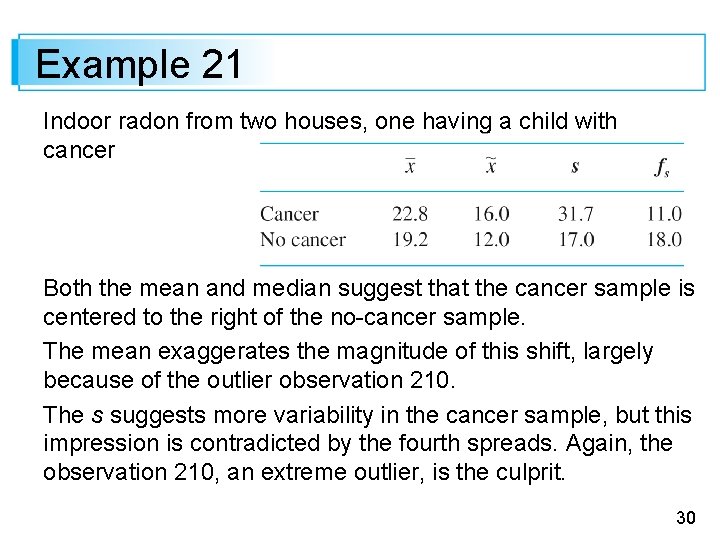
Example 21 Indoor radon from two houses, one having a child with cancer Both the mean and median suggest that the cancer sample is centered to the right of the no-cancer sample. The mean exaggerates the magnitude of this shift, largely because of the outlier observation 210. The s suggests more variability in the cancer sample, but this impression is contradicted by the fourth spreads. Again, the observation 210, an extreme outlier, is the culprit. 30

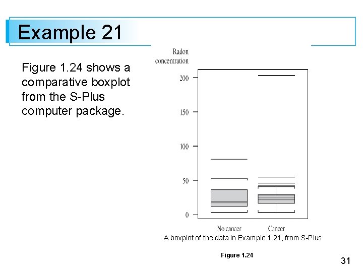
Example 21 Figure 1. 24 shows a comparative boxplot from the S-Plus computer package. A boxplot of the data in Example 1. 21, from S-Plus Figure 1. 24 31

Example 21 The no-cancer box is stretched out compared with the cancer box (fs = 18 vs. fs = 11), and the positions of the median lines in the two boxes show much more skewness in the middle half of the no-cancer sample than the cancer sample. Outliers are represented by horizontal line segments, and there is no distinction between mild and extreme outliers. 32