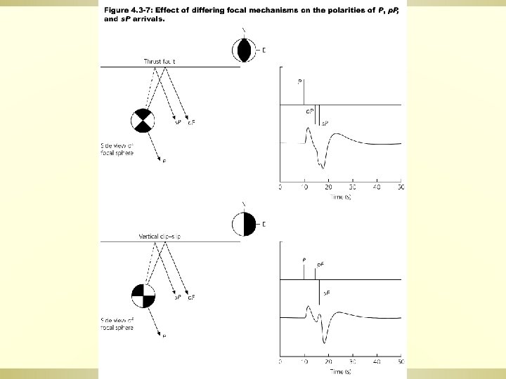
Waveform modelling Last Time Seismic wave II PhaseGroup


: effect of reflections and conversions, geometric spreading Q(w): attenuation")


")
, is comparable to the wavelength")

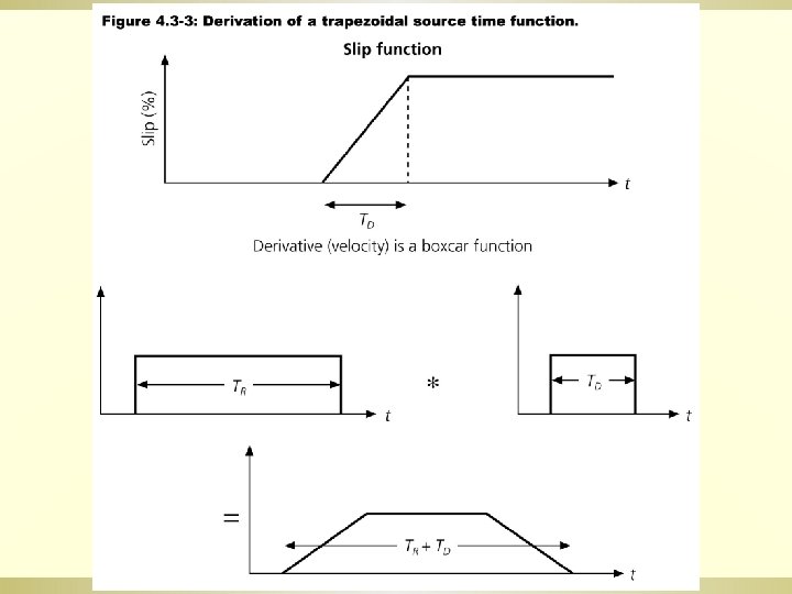
. A Trapezoidal time function is")

, which includes")


 F-k (Lupei Zhu, http: //www.")
- Slides: 44
Waveform modelling 波形模拟
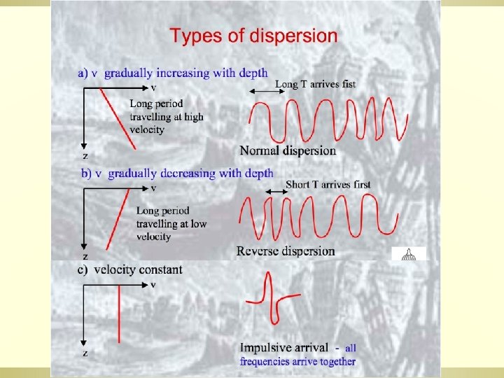
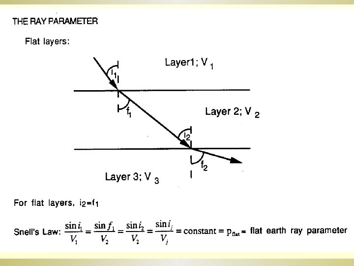
Last Time ß ß Seismic wave II (Phase/Group velocity, Dispersion, Attenuation, Fermat’s principle, Snell’s law, Huygens’ principle) Normal modes (Normal modes of string, Normal modes of a sphere, Observations of normal modes)
Free oscillations m=0; n=0; l=0, Period ~20 minutes m=+-2; n=0; l=3, Period~36 minutes
Generated by the great June 9, 1994 deep focus Bolivia earthquake. Recorded at Pasadena, California.
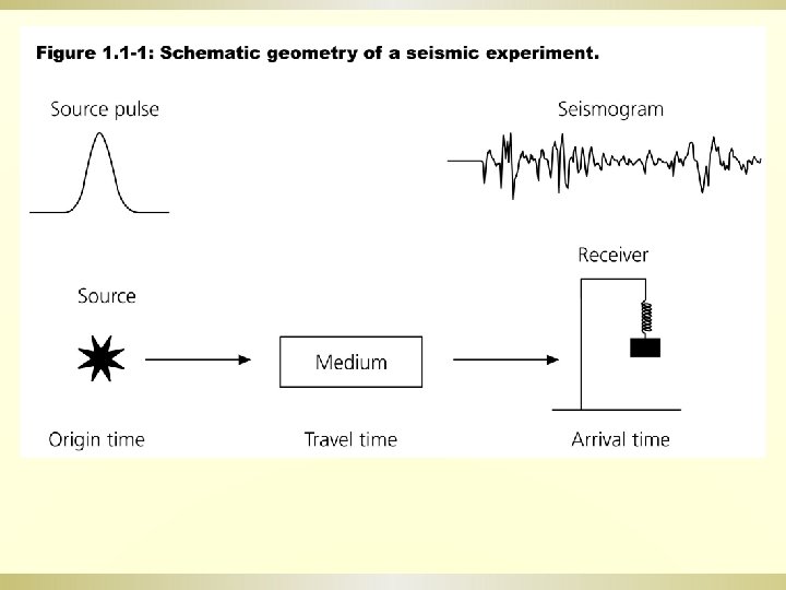
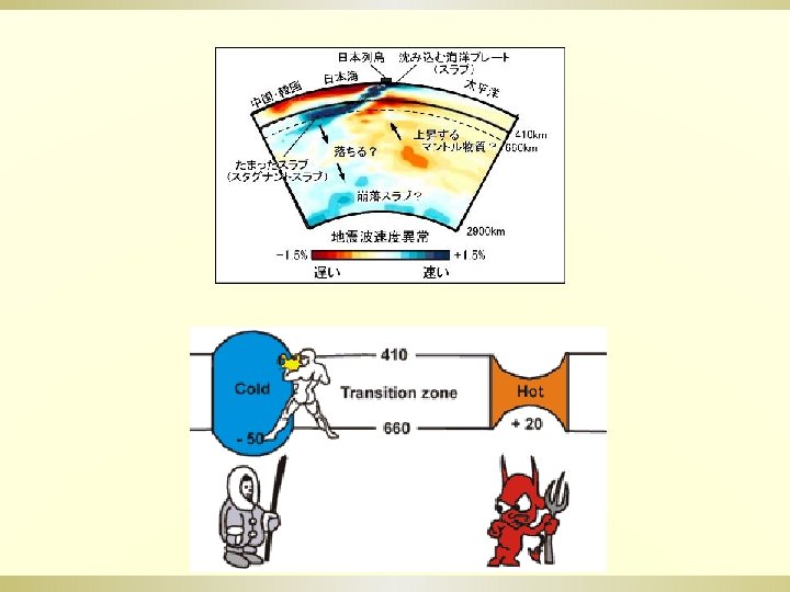
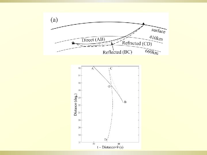
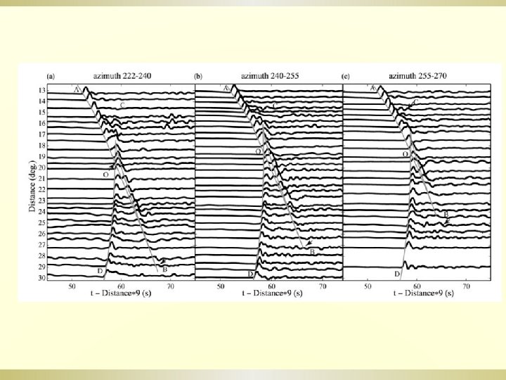
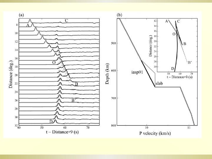
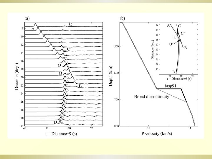
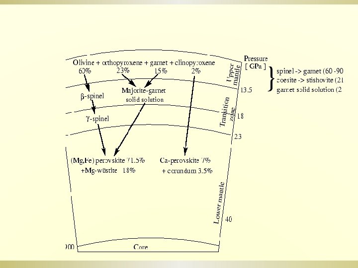
This time ß Waveform modeling Þ Þ Þ Basic model Source time function Body wave modeling Green’s functions An example on 660 -km discntinuity
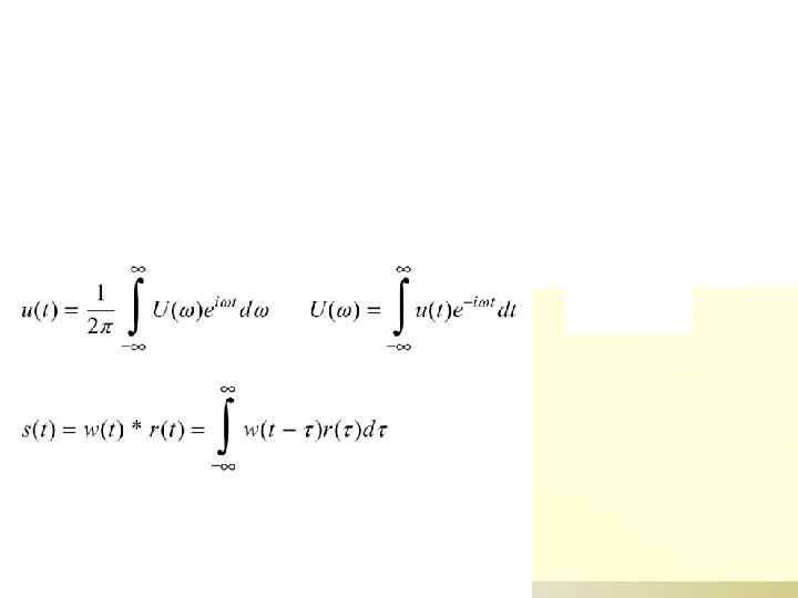
E(w): effect of reflections and conversions, geometric spreading Q(w): attenuation
More on convolution ß A convolution is an integral that expresses the amount of overlap of one function g as it is shifted over another function f (Wolfram)
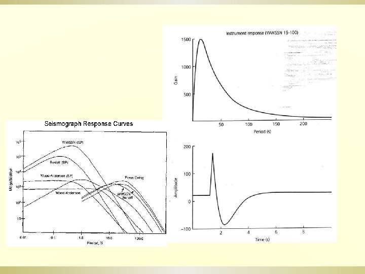
Impulse response of a longperiod WWSSN seismometers in both time and frequency domains.
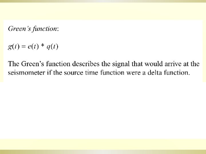
The simplest case: a delta function.
The simplest case: a delta function.
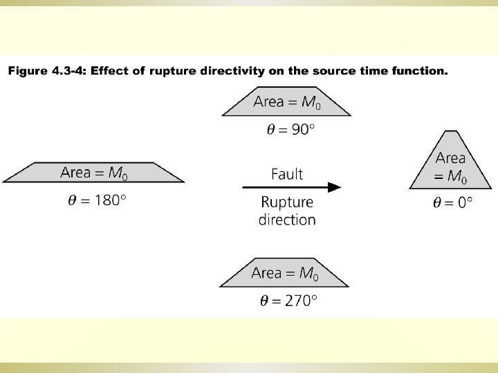
zebu. uoregon. edu/~js/space/ lectures/lec 05. html Moving wave sources Doppler shift Stationary source Source moving to the left
Doppler shift 1 2 3 1 Lower pitch For example, approaching siren has a higher pitch than a receding siren 2 3 Higher pitch
2004 Mw 9. 3 Sumatra earthquake (Ni et al. , Nature, 2005)
For example, a 10 km-long fault (M 6 earthquake), is comparable to the wavelength of 1 s body Wave propagating at 8 km/s, but very small compared with the 200 km wavelength of a 50 s surface wave propagating at 4 km/s. However, a 300 km-long fault for a magnitude 8 earthquake would be a finite source for surface waves.
Body wave modeling
Earthquake near the Sumatra trench (Stein and Wiens, 1986). A Trapezoidal time function is assumed.
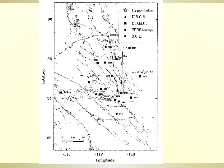
Near source strong motion records is needed for inversions of source time functions (Stein and Kroeger, 1980).
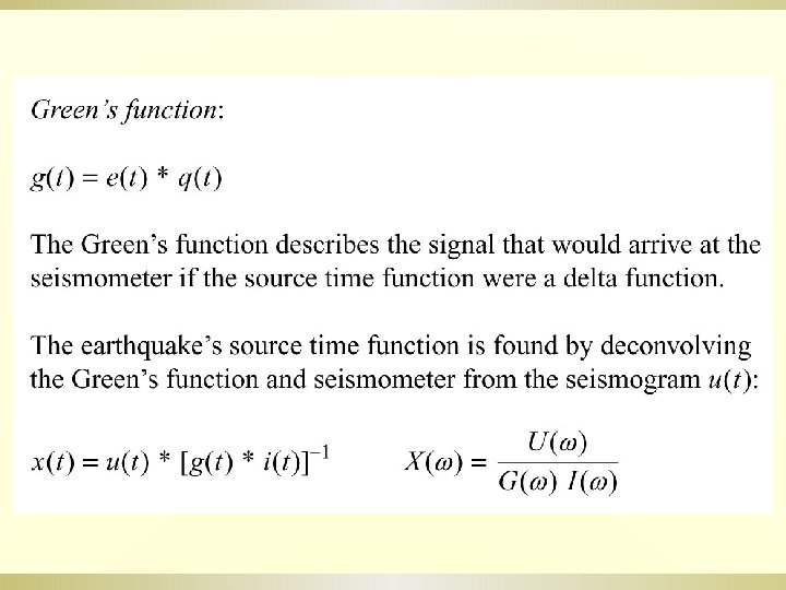
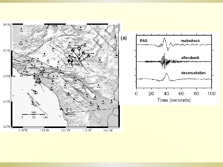
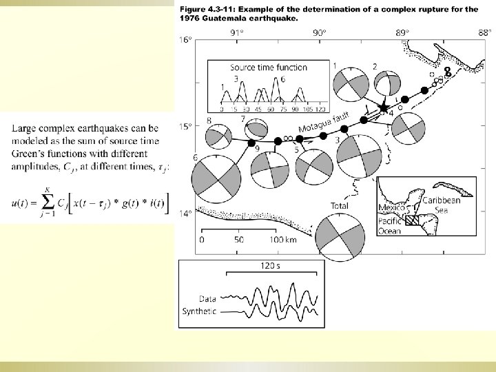
Green’s function ß ß The impulse response of the system (the Earth), which includes attenuation, propagation, instrument, and radiation pattern effects. If the earthquake is small enough, we can consider its waveform as an ‘empirical Green’s function’
Ammon et al. , 2006
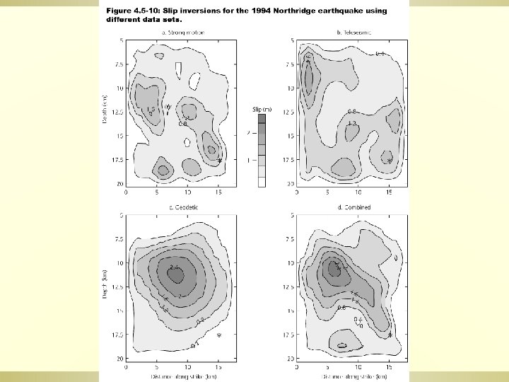
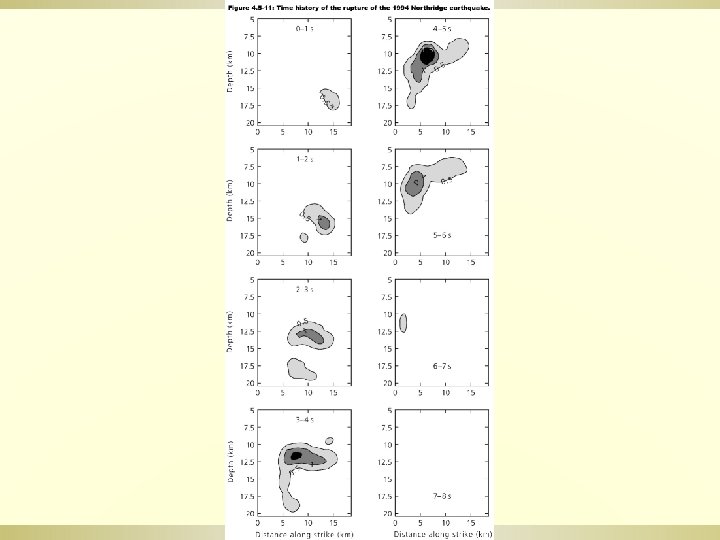
Joint geodetic and seismological EQ studies Both data types are complementary. e. g. , Seismic waves have an ambiguity in distinguishing the true fault plane and the auxiliary plane. But the geodetic data do not. The geodetic data depend on the difference in position before and after an earthquake (i. e. , static displacement). So we have to count on seismograms to figure out how the rupture evolved during an earthquake.
http: //www. seisdmc. ac. cn Wang & Niu, 2010, JGR
Tools for synthetic seismogram ß ß Qseis (Rongjiang Wang) F-k (Lupei Zhu, http: //www. eas. slu. edu/People/LZhu/home. html ß ß ) FD (http: //geodynamics. org/cig) SEM (http: //geodynamics. org/cig)