Water Resources Development and Management Optimization Nonlinear Programming
 CVEN 5393")


 is convex if it “bend upward”. To")


 If f (x 1, x")

 Nonlinear")


 Convex programming The assumptions in convex programming are These assumptions are enough to")
 Separable programming ( a special case of convex programming) Separable programming is a")
 Nonconvex programming")


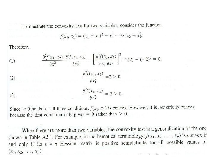
 is concave by the convexity test.")

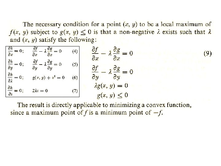
 Conditions for Constrained Optimization The necessary and sufficient conditions that must")
 Conditions ?")


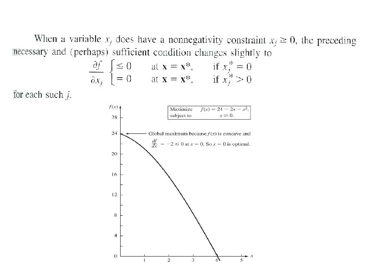
 conditions for general case These conditions are sufficient if f is concave")


")


 is")


 is the optimal solution")
 HUGHES-MCMAKEE-NOTESCHAPTER 11. PDF HUGHES-MCMAKEE-NOTESCHAPTER 08.")
- Slides: 72
Water Resources Development and Management Optimization (Nonlinear Programming & Time Series Simulation) CVEN 5393 Apr 11, 2011
Acknowledgements • Dr. Yicheng Wang (Visiting Researcher, CADSWES during Fall 2009 – early Spring 2010) for slides from his Optimization course during Fall 2009 • Introduction to Operations Research by Hillier and Lieberman, Mc. Graw Hill
Today’s Lecture • Nonlinear Programming • Time Series Simulation • R-resources / demonstration
NONLINEAR PROGRAMMING
IV. Nonlinear Programming A nonlinear programming example x 1+x 2+x 3 ≤ Q x 1,x 2,x 3 ≥ 0
In one general form, the nonlinear programming problem is to find x = (x 1, x 2, …, xn) so as to Many types of nonlinear programming problems. Different algorithms for different programming problems.
1. Graphical Illustration of Nonlinear Programming C C
D E
A local maximum need not be a global maximum C B A D E F Nonlinear Programming algorithms generally can not distinguish between a local optimal solution and a global optimal solution.
2. Convexity Convex or concave functions of a single variable H A L B
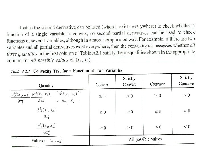
The geometric interpretation indicates that f (x) is convex if it “bend upward”. To be more precise, if f (x) possesses a second derivative everywhere, then f (x) is convex if and only if for all possible values of x In terms of the second derivative of the function, the convexity test is summarized below.
M N A convex function A strictly convex function T A concave function A strictly concave function
A function that is both convex and concave A function that is neither convex nor concave
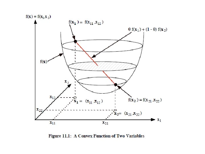
Convex or concave functions of several variables
Two important properties of convex or concave functions (1) If f (x 1, x 2, ---, xn) is a convex function, then g(x 1, x 2, ---, xn) = - f (x 1, x 2, ---, xn) is a concave function, and vice versa (2) The sum of convex functions is a convex function, and the sum of concave functions is a concave function.
Convex Sets
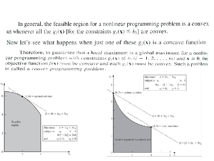
Condition for a local optimal solution to be a global optimal solution (1) Nonlinear programming problems without constraints If a nonlinear programming problem has no constraints, the objective function being concave guarantees that a local maximum is a global maximum (Similarly, the objective function being convex ensures that a local minimum is a global minimum). (2) Nonlinear programming problems with constraints If a nonlinear programming problem has constraints, both the objective function being concave and the feasible region being a convex set guarantees that a local maximum is a global maximum (Similarly, both the objective function being convex and the feasible region being a convex set ensures that a local minimum is a global minimum). For any linear programming problem, its linear objective function is both convex and concave and its feasible region is a convex set, so its optimal solution is certainly a global optimal solution.
B C D A E
3. Classical Optimization Methods Unconstrained optimization of a function of a single variable If (If f (x) is strictly convex in the vicinity of x*, is the necessary and sufficient condition for the solution x = x* to be a local minimum) Global minimum: point A Global maximum: point E If f (x) is strictly convex everywhere, there is only one local minimum, which is the global minimum B A C D E
Unconstrained optimization of a function of several variables
Constrained optimization with equality constraints For any feasible solution, we have
Example: Solutions: f=2 f = -2
4. Types of Nonlinear Programming Problems Nonlinear programming problems come in many different shapes and forms. No single algorithm can solve all these different types of problems. Algorithms have been developed for various special types of nonlinear programming problems. (1) Unconstrained optimization
(2) Convex programming The assumptions in convex programming are These assumptions are enough to ensure that a local maximum is a global maximum. (3) Linearly constrained optimization ( a special case of convex programming) (4) Quadratic Programming ( a special case of linearly constrained optimization )
(4) Separable programming ( a special case of convex programming) Separable programming is a special case of convex programming, where the one additional assumption is
(5) Nonconvex programming
5. One-Variable Unconstrained Optimization One-Dimensional Search Procedure A number of efficient one-dimensional search procedure available. For example, Sequential-Search Techniques, Three-Point Interval Search, Fibonacci Search, Golden. Mean Search, etc. Next, only one of the sequential-search techniques, the Midpoint Method, is introduced. The idea behind the one-dimensional search procedure is a very intuitive one. This procedure checks whether the slope is positive or negative at a trial solution. As shown in the figure, x* is the optimum. If the first derivative at a particular value of x is positive, then x* must be larger than this x, so this x becomes a lower bound. Conversely, if the first derivative at a particular value of x is negative, then x* must be smaller than this x, so this x becomes a upper bound.
The entire process of the midpoint method is summarized next, given the notation.
Example:
5. Multivariable Unconstrained Optimization One-variable unconstrained optimization : the first derivative of the objective function is used to select one of the just two possible directions (increase x or decrease x) in which to move from the current trial solution to the next one. The goal is to reach a point eventually where the first derivative is 0. Multivariable unconstrained optimization : There are innumerable possible directions in which to move. The gradient of the objective function is used to select the specific direction in which to move. The goal is to reach a point eventually where all the partial derivatives are 0. The gradient at a specific point x=x' is the vector whose elements are the respective partial derivatives at x=x' , so that
Gradient Search Procudure The gradient search procedure is to keep moving in the direction of the gradient from the current trial solution, not stopping until f (x) stops increasing. This stopping point would be the next trial solution, so the gradient then would be recalculated to determine the new direction in which to move. With this approach, each iteration involves changing the current trial solution x' as follows.
Summary of the Gradient Search Procedure
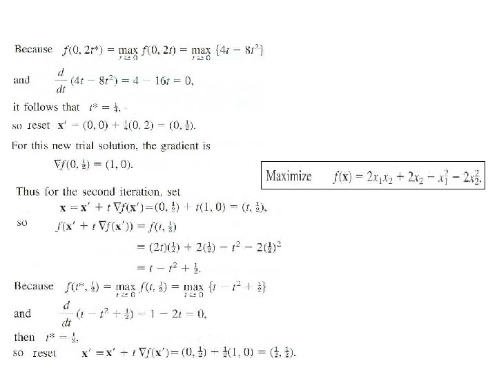
Example: It can be verified that f (x) is concave by the convexity test. To begin the gradient search procedure, x = (0, 0) is selected as the initial trial solution. The gradient at x = (0, 0) is To begin the first iteration, set and then substitute these expressions into f (x) to obtain
By continuing in this way, the subsequent solutions can be obtained as shown in the figure. Because these points are converging to x*=(1, 1), this solution is the optimal solution, as verified by the fact that However, because this converging sequence of trial solutions never reaches its limit, the procedure actually will stop somewhere slightly below (1, 1) as its final approximation of x*.
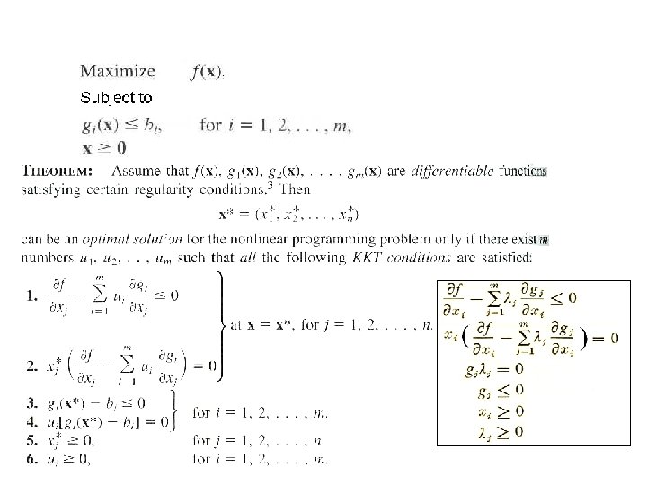
6. Karush-Kuhn-Tucker (KKT) Conditions for Constrained Optimization The necessary and sufficient conditions that must be satisfied by an optimal solution for a nonlinear programming problem.
What are Karush-Kuhn-Tucker (KKT) Conditions ?
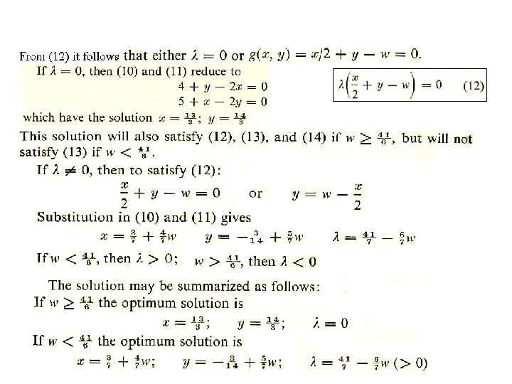
Example:
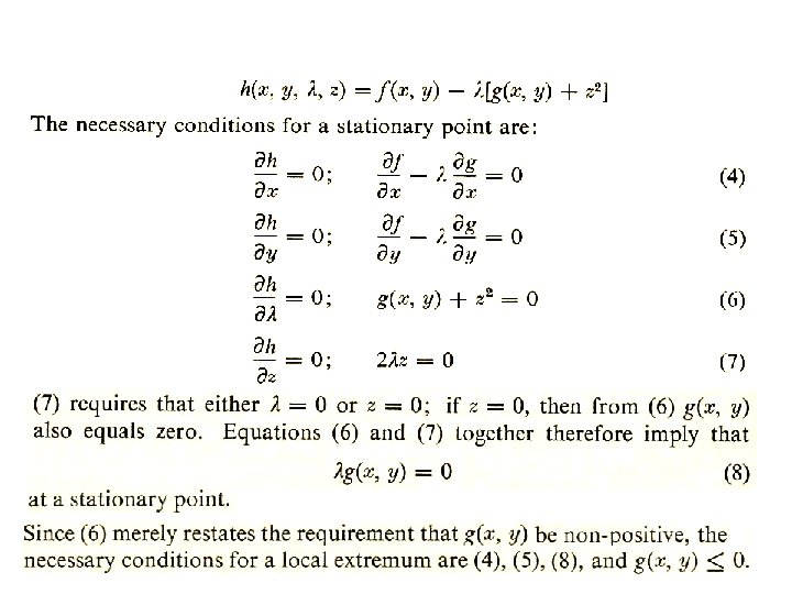
The necessary conditions if x and y are to be nonnegative are
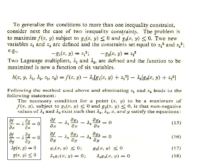
Karush-Kuhn-Tucker (KKT) conditions for general case These conditions are sufficient if f is concave and gi are all convex.
7. Quadratic Programming The quadratic programming problem differs from the linear programming problem only in that the objective function also includes and The matrix form of a quadratic programming problem is , say, Q is a symmetrical matrix. The algebraic form of the objective function of this quadratic programming problem is
Example: To illustrate the notation, consider the following example of a quadratic programming problem. In this case, f (x 1, x 2) can be rewritten as
Algorithm for quadratic programming KKT conditions for quadratic programming g 1(x 1, x 2) = x 1 + 2 x 2
We have
We now have the desired convenient form for the entire set of conditions shown below. This form is particularly convenient because, except for the complementarity constraint, these conditions are linear programming constraints. For any quadratic programming problem, its KKT conditions can be reduced to this same convenient form containing just linear programming constraints plus one complementarity constraint. In matrix notation, this general form is where the elements of the column vector u are Lagrange multipliers and the elements of the column vectors y and v are slack variables. The original problem is reduced to the equivalent problem of finding a feasible solution to these constraints.
Modified simplex method The KKT conditions for quadratic programming are nothing more than linear programming constraints, except for the complementary constrain. The complementary constraint simply implies that it is not permissible for both complementary variables of any pair to be basic variables when BF solutions are considered. As a result, the problem reduces to finding an initial BF solution to any linear programming problem that has the constraints shown below (obtained from the KKT conditions for quadratic programming ). In the simple case where c. T ≤ 0 and b ≥ 0, we can easily find a feasible solution which satisfies the above constraints and thus is the optimal solution for the quadratic programming problem. In the case where c. T > 0 or b < 0, we have to introduce artificial variables as we do for the Big M method or the two-phase method.
So we use phase 1 of the two-phase method to find a BF solution satisfying the constraints obtained from the KKT conditions. Specifically, we apply the simplex method with one modification to the following linear programming problem subject to the linear programming constraints obtained from the KKT conditions, but with the artificial variables zj included. The one modification in the simplex method is the following change in the procedure for selecting an entering basic variable.
Example to illustrate the modified simplex method As can be verified from the convexity test, f (x 1, x 2) is strictly concave,so the modified simplex method can be applied. After the artificial variables are introduced, the linear programming problem to be addressed by the modified simplex method is
For each of the three pairs of complementary variables whenever one of the two variables already is a basic variable, the other variable is excluded as a candidate for the entering basic variable. The initial set of basic variables gives an initial BF solution that satisfies the complementary constraint. The table shows the results of applying the modified simplex method to this example. The first exhibits the initial system of equations after converting from minimizing Z to maximizing –Z and algebraically eliminating the initial basic variables form Eq. (0). The three iterations proceed just as for the regular simplex method, except for eliminating certain candidates for the entering basic variable because of the restricted-entry rule.
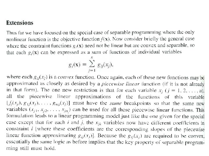
8. Separable Programming In Separable programming , it is assumed that the objective function f(x) is concave, that each of the constraint functions gi(x) is convex, and that all these functions are separable functions. However, to simplify the discussion, we focus here on the special case where the convex and separable gi(x) are linear functions, just as for linear programming. Thus only the objective function requires special treatment. A concave and separable function can be expressed as a sum of concave functions of individual variables. so that each fj(xj) has a shape such as either case shown in the figure below over the feasible range of values of xj.
In case 1, the slope decreases only at certain breakpoints, so that fj(xj) is a piecewise linear function (a sequence of connected line segments). In case 2, the slope may decrease continuously as xj increases, so that fj(xj) is a general concave function. Any such function can be approximated as closely as desired by a piecewise linear function.
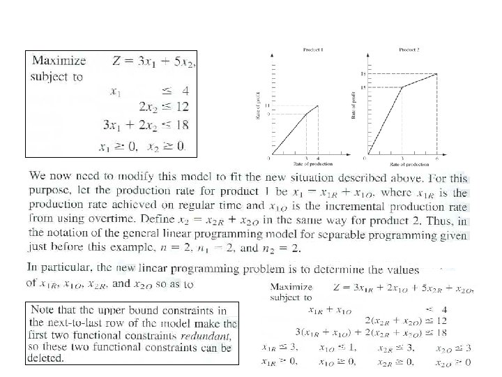
Reformulation as a Linear Programming Problem The key to rewriting a piecewise linear function as a linear function is to use a separate variable for each line segment. To illustrate, consider the piecewise linear function in case 1 or the approximating piecewise linear function in case 2 Introduce three new variables xj 1, xj 2, and xj 3 and set where
Special restriction permits
To write down the complete model in the preceding notation, let nj be the number of line segments in fj (xj), so that
Unfortunately, the special restriction does not fit into the required format for linear programming constraints. However, our fj (xj) are assumed to be concave so that an algorithm for maximizing f (x) automatically gives the highest priority to using xj 1 when increasing xj from zero, the next highest priority to using xj 2, and so on, without even including the special restriction explicitly in the model. This observation leads to the following key property.
After obtaining an optimal solution for the model, you then calculate for j = 1, 2, …, n in order to identify an optimal solution for the original separable programming program or its piecewise linear approximation.
Example:
(x 1=4 and x 2=3) is the optimal solution
NONLINEAR PROGRAMMING & PIECEWISE LINEAR LP (PROF. MCMAKEE NOTES) HUGHES-MCMAKEE-NOTESCHAPTER 11. PDF HUGHES-MCMAKEE-NOTESCHAPTER 08. PDF