Volatility in Financial Time Series Autoregressive Conditional Heteroskedasticity

Volatility in Financial Time Series Autoregressive Conditional Heteroskedasticity

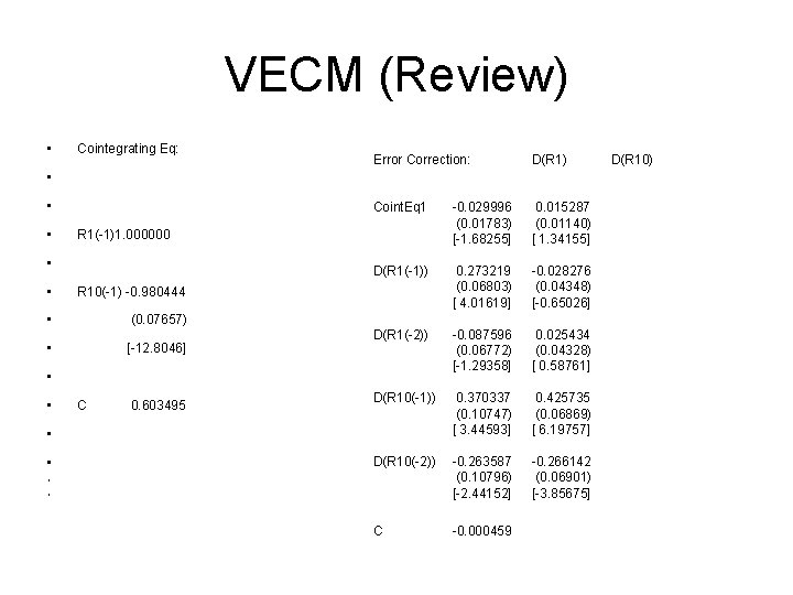
VECM (Review) • Cointegrating Eq: Error Correction: D(R 1) Coint. Eq 1 -0. 029996 (0. 01783) [-1. 68255] 0. 015287 (0. 01140) [ 1. 34155] D(R 1(-1)) 0. 273219 (0. 06803) [ 4. 01619] -0. 028276 (0. 04348) [-0. 65026] D(R 1(-2)) -0. 087596 (0. 06772) [-1. 29358] 0. 025434 (0. 04328) [ 0. 58761] D(R 10(-1)) 0. 370337 (0. 10747) [ 3. 44593] 0. 425735 (0. 06869) [ 6. 19757] D(R 10(-2)) -0. 263587 (0. 10796) [-2. 44152] -0. 266142 (0. 06901) [-3. 85675] C -0. 000459 • • • R 1(-1)1. 000000 • • R 10(-1) -0. 980444 • (0. 07657) • [-12. 8046] • • C 0. 603495 • • D(R 10)

Introduction • Assess Maximum Likelihood estimation. • Non linear models – Three forms – Testing • General tests • Specific tests • Models for Volatility – Simple forms – ARCH – GARCH • Constraints and limitations

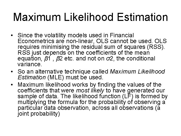
Maximum Likelihood Estimation • Since the volatility models used in Financial Econometrics are non-linear, OLS cannot be used. OLS requires minimising the residual sum of squares (RSS). RSS just depends on the coefficients of the mean equation, β 1 , β 2 etc. and not on σ2, the conditional variance. • So an alternative technique called Maximum Likelihood Estimation (MLE) must be used. • Maximum likelihood works by finding the values of the coefficients that were most likely to have generated our sample of data. The likelihood function (LF) is formed by multiplying the formula for the probability of observing a particular data observation, across all observations (a joint probability)

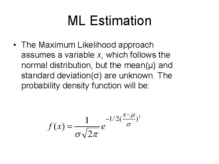
ML Estimation • The Maximum Likelihood approach assumes a variable x, which follows the normal distribution, but the mean(μ) and standard deviation(σ) are unknown. The probability density function will be:

ML Estimation • To determine the value of the mean, we need to maximise the likelihood function, or joint probability density. • It is easier to use the log-likelihood though, as the value that maximises the likelihood function also maximises the log-likelihood function. • It is then a matter of differentiating with respect to the mean μ, to find the maximum value of the log-likelihood function and setting this equal to zero.

Application to simple regression model • Assuming that the error term is normally distributed with zero mean and standard deviation σ. • It is then a process of forming the log-likelihood function and the values for the constant and slope parameter that maximise this function are exactly the same as those obtained by OLS. • However the estimate of σ is slightly different.

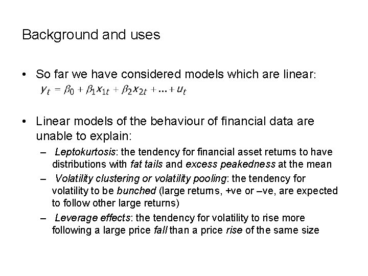
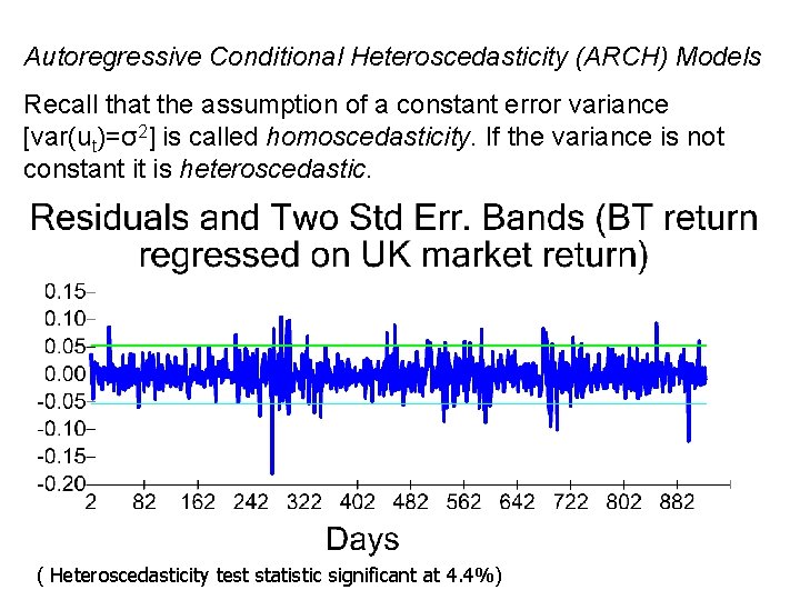
Background and uses • So far we have considered models which are linear: • Linear models of the behaviour of financial data are unable to explain: – Leptokurtosis: the tendency for financial asset returns to have distributions with fat tails and excess peakedness at the mean – Volatility clustering or volatility pooling: the tendency for volatility to be bunched (large returns, +ve or –ve, are expected to follow other large returns) – Leverage effects: the tendency for volatility to rise more following a large price fall than a price rise of the same size

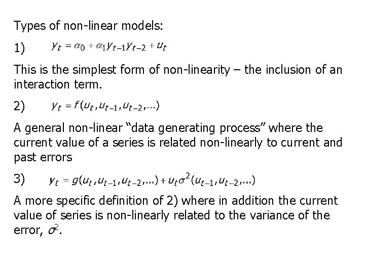
Types of non-linear models: 1) This is the simplest form of non-linearity – the inclusion of an interaction term. 2) A general non-linear “data generating process” where the current value of a series is related non-linearly to current and past errors 3) A more specific definition of 2) where in addition the current value of series is non-linearly related to the variance of the error, σ2.

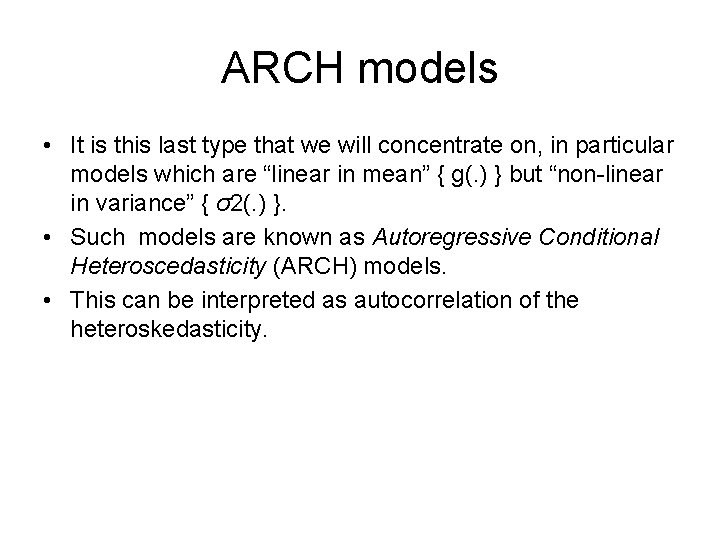
ARCH models • It is this last type that we will concentrate on, in particular models which are “linear in mean” { g(. ) } but “non-linear in variance” { σ2(. ) }. • Such models are known as Autoregressive Conditional Heteroscedasticity (ARCH) models. • This can be interpreted as autocorrelation of the heteroskedasticity.

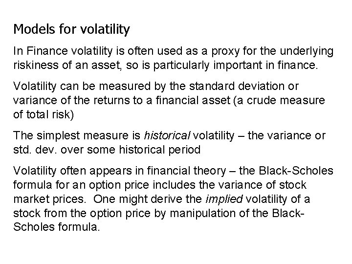
Models for volatility In Finance volatility is often used as a proxy for the underlying riskiness of an asset, so is particularly important in finance. Volatility can be measured by the standard deviation or variance of the returns to a financial asset (a crude measure of total risk) The simplest measure is historical volatility – the variance or std. dev. over some historical period Volatility often appears in financial theory – the Black-Scholes formula for an option price includes the variance of stock market prices. One might derive the implied volatility of a stock from the option price by manipulation of the Black. Scholes formula.

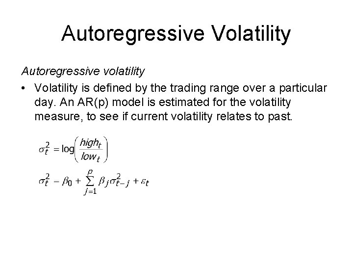
Autoregressive Volatility Autoregressive volatility • Volatility is defined by the trading range over a particular day. An AR(p) model is estimated for the volatility measure, to see if current volatility relates to past.

Autoregressive Conditional Heteroscedasticity (ARCH) Models Recall that the assumption of a constant error variance [var(ut)=σ2] is called homoscedasticity. If the variance is not constant it is heteroscedastic. ( Heteroscedasticity test statistic significant at 4. 4%)

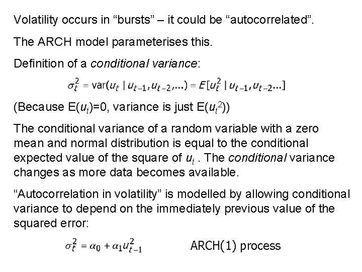
Volatility occurs in “bursts” – it could be “autocorrelated”. The ARCH model parameterises this. Definition of a conditional variance: (Because E(ut)=0, variance is just E(ut 2)) The conditional variance of a random variable with a zero mean and normal distribution is equal to the conditional expected value of the square of ut. The conditional variance changes as more data becomes available. “Autocorrelation in volatility” is modelled by allowing conditional variance to depend on the immediately previous value of the squared error: ARCH(1) process

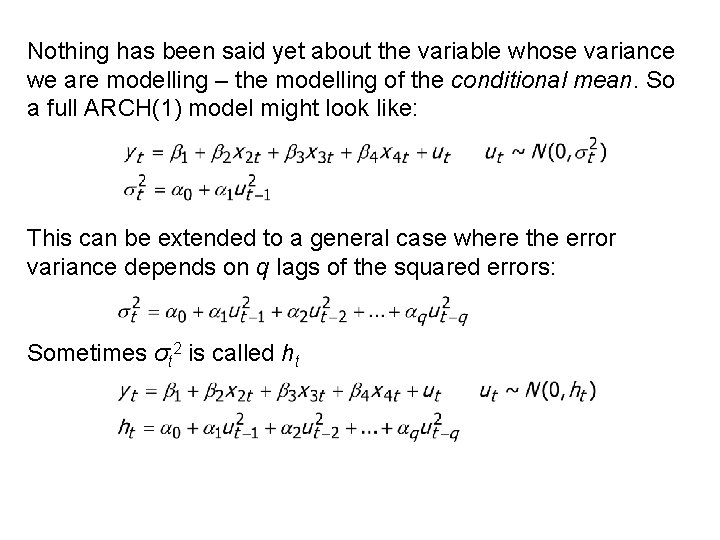
Nothing has been said yet about the variable whose variance we are modelling – the modelling of the conditional mean. So a full ARCH(1) model might look like: This can be extended to a general case where the error variance depends on q lags of the squared errors: Sometimes σt 2 is called ht

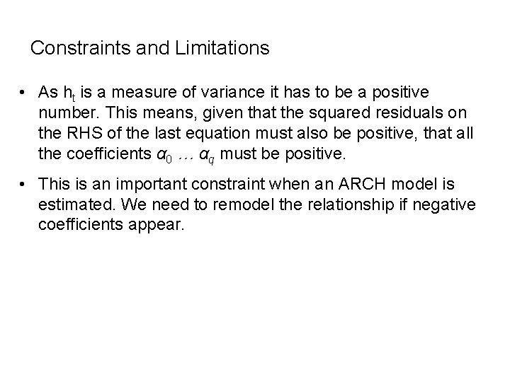
Constraints and Limitations • As ht is a measure of variance it has to be a positive number. This means, given that the squared residuals on the RHS of the last equation must also be positive, that all the coefficients α 0 … αq must be positive. • This is an important constraint when an ARCH model is estimated. We need to remodel the relationship if negative coefficients appear.

Testing for ARCH • Run the regression model that you wish to investigate and save the residuals. • Compute the square of the residuals and regress them on q lags of themselves: • Note the R 2 from this regression. • Compute the test statistic T. R 2 (where T is the number of observations in the sample. This has a Chi 2 (q) distribution. The null hypothesis is no “ARCH effects”, so if T. R 2 is less than the Chi 2 critical value we accept the null hypothesis of no ARCH effects in the model.

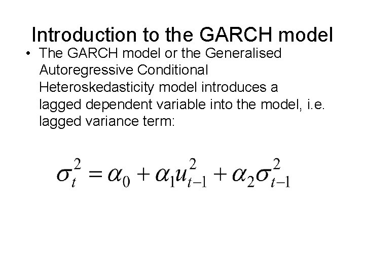
Introduction to the GARCH model • The GARCH model or the Generalised Autoregressive Conditional Heteroskedasticity model introduces a lagged dependent variable into the model, i. e. lagged variance term:

GARCH Model • The GARCH model has been shown to have a better performance than the ARCH model using a smaller number of terms, i. e. it is more parsimonious • Often a GARCH (1, 1) model is sufficient to explain the volatility in a financial time series.

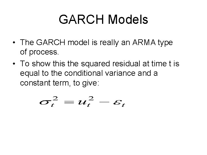
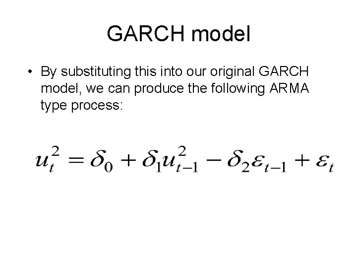
GARCH Models • The GARCH model is really an ARMA type of process. • To show this the squared residual at time t is equal to the conditional variance and a constant term, to give:

GARCH model • By substituting this into our original GARCH model, we can produce the following ARMA type process:

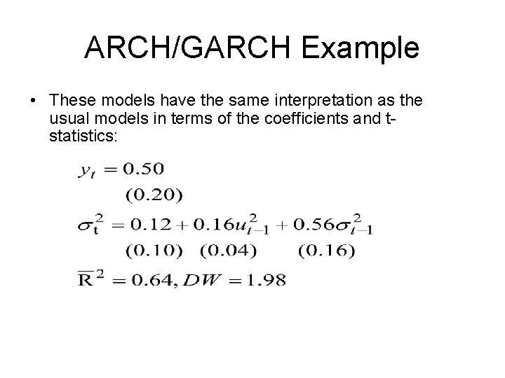
ARCH/GARCH Example • These models have the same interpretation as the usual models in terms of the coefficients and tstatistics:

ARCH Example • The first step involves estimating the mean, often this involves regressing the variable of interest against a constant, the resulting error term (u) is used to produce the conditional variance term in the resulting GARCH model. • However the mean equation can include other terms, often ARIMA models are used. • In the previous slide the GARCH model has significant variables, which are correctly signed and the diagnostic tests are passed

ARCH Example • The use of GARCH models is not only required to ensure the model is well specified, it can also be used forecasting. • GARCH models have proven to be particularly useful at forecasting returns on risky assets.

Conclusion • Volatility is important in finance as it represents risk and is a particular feature of financial data. • Many assets exhibit volatility clustering, such that there is autocorrelation in the heteroskedasticity. • The ARCH model is an important way of modelling this phenomenon • The GARCH model has better time series properties than the ARCH model.