Visual Sensing and Perception ECE 383 MEMS 442

Visual Sensing and Perception ECE 383 / MEMS 442: Intro to Robotics and Automation Kris Hauser

Agenda • A high-level overview of visual sensors and common geometric representations • Core concepts • Camera / projective geometry • Working with images • Point clouds • Readings: Computer Vision: Algorithms and Applications Ch 2. 1 and 12. 2 (http: //szeliski. org/Book/drafts/Szeliski. Book_20100903_draft. pdf)

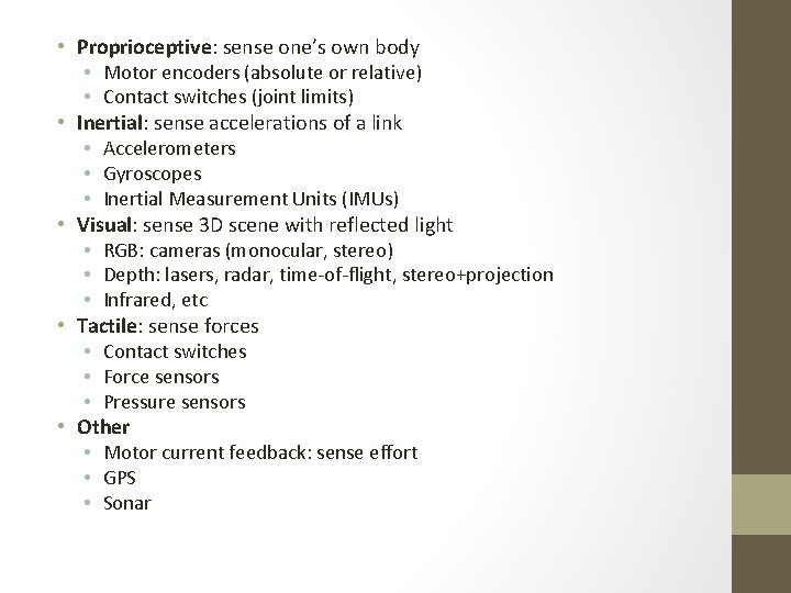
• Proprioceptive: sense one’s own body • Motor encoders (absolute or relative) • Contact switches (joint limits) • Inertial: sense accelerations of a link • Accelerometers • Gyroscopes • Inertial Measurement Units (IMUs) • Visual: sense 3 D scene with reflected light • RGB: cameras (monocular, stereo) • Depth: lasers, radar, time-of-flight, stereo+projection • Infrared, etc • Tactile: sense forces • Contact switches • Force sensors • Pressure sensors • Other • Motor current feedback: sense effort • GPS • Sonar

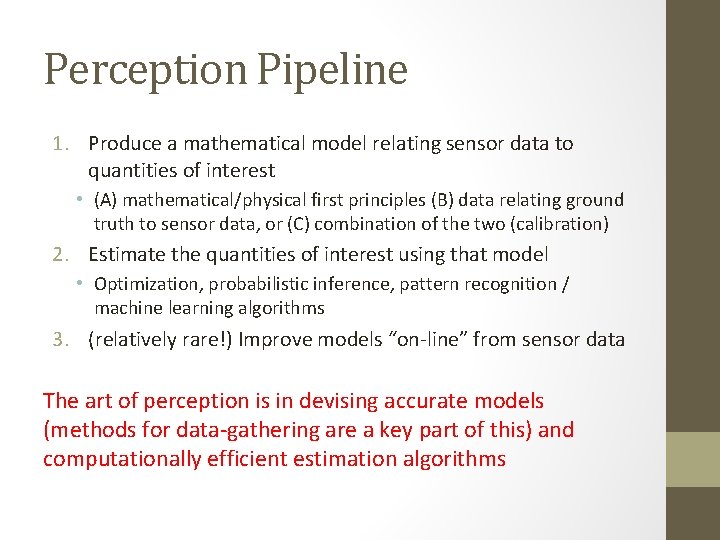
Perception Pipeline 1. Produce a mathematical model relating sensor data to quantities of interest • (A) mathematical/physical first principles (B) data relating ground truth to sensor data, or (C) combination of the two (calibration) 2. Estimate the quantities of interest using that model • Optimization, probabilistic inference, pattern recognition / machine learning algorithms 3. (relatively rare!) Improve models “on-line” from sensor data The art of perception is in devising accurate models (methods for data-gathering are a key part of this) and computationally efficient estimation algorithms

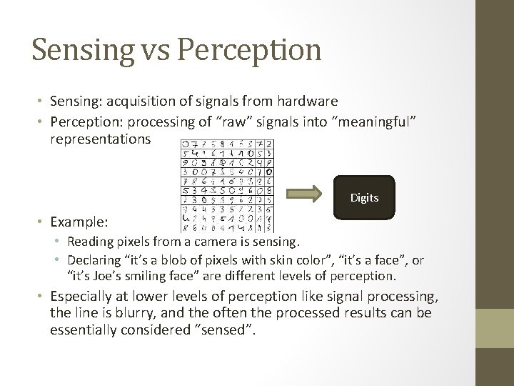
Sensing vs Perception • Sensing: acquisition of signals from hardware • Perception: processing of “raw” signals into “meaningful” representations Digits • Example: • Reading pixels from a camera is sensing. • Declaring “it’s a blob of pixels with skin color”, “it’s a face”, or “it’s Joe’s smiling face” are different levels of perception. • Especially at lower levels of perception like signal processing, the line is blurry, and the often the processed results can be essentially considered “sensed”.

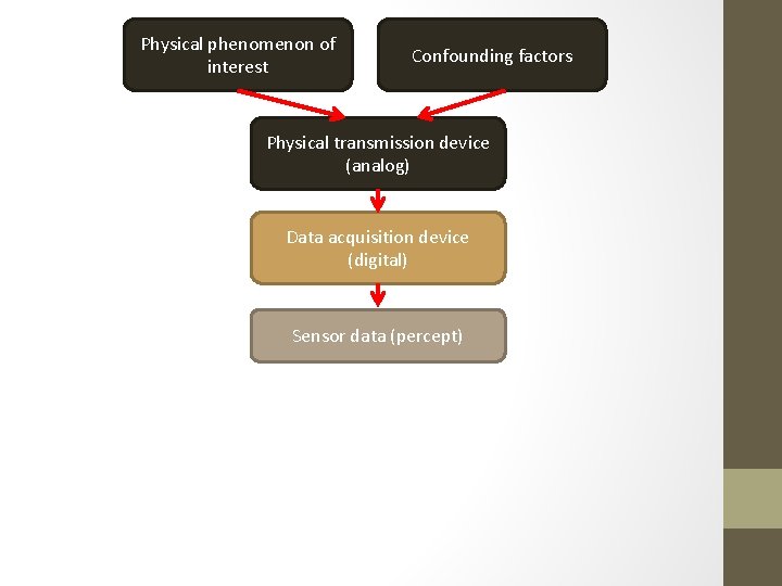
Physical phenomenon of interest Confounding factors Physical transmission device (analog) Data acquisition device (digital) Sensor data (percept)

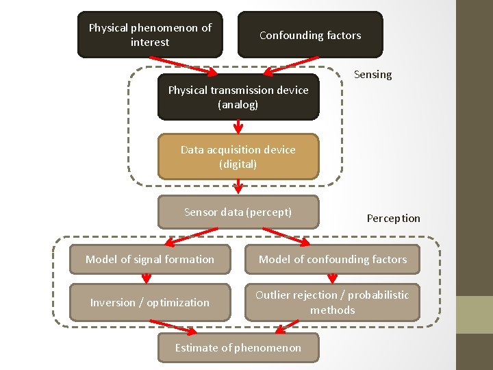
Physical phenomenon of interest Confounding factors Sensing Physical transmission device (analog) Data acquisition device (digital) Sensor data (percept) Perception Model of signal formation Model of confounding factors Inversion / optimization Outlier rejection / probabilistic methods Estimate of phenomenon

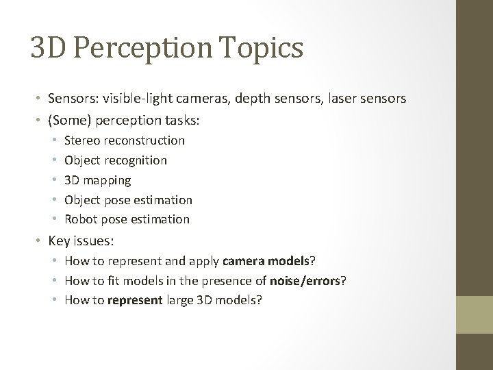
3 D Perception Topics • Sensors: visible-light cameras, depth sensors, laser sensors • (Some) perception tasks: • • • Stereo reconstruction Object recognition 3 D mapping Object pose estimation Robot pose estimation • Key issues: • How to represent and apply camera models? • How to fit models in the presence of noise/errors? • How to represent large 3 D models?

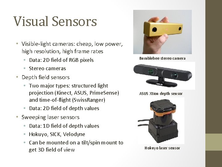
Visual Sensors • Visible-light cameras: cheap, low power, high resolution, high frame rates • Data: 2 D field of RGB pixels • Stereo cameras • Depth field sensors • Two major types: structured light projection (Kinect, ASUS, Prime. Sense) and time-of-flight (Swiss. Ranger) • Data: 2 D field of depth values • Sweeping laser sensors • Data: 1 D field of depth values • Hokuyo, SICK, Velodyne • Can be mounted on a tilt/spin mount to get 3 D field of view Bumblebee stereo camera ASUS Xtion depth sensor Hokuyo laser sensor

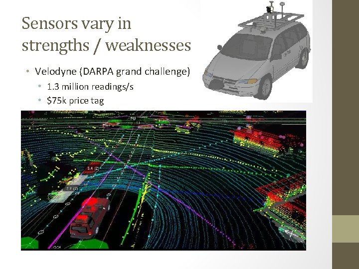
Sensors vary in strengths / weaknesses • Velodyne (DARPA grand challenge) • 1. 3 million readings/s • $75 k price tag

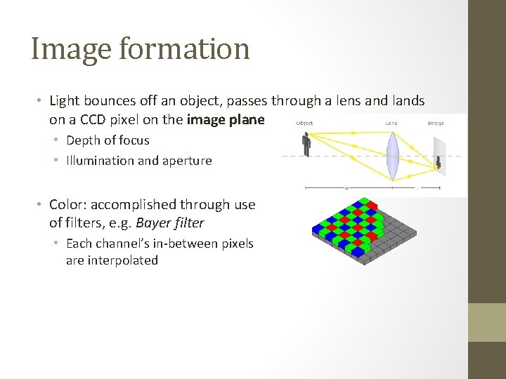
Image formation • Light bounces off an object, passes through a lens and lands on a CCD pixel on the image plane • Depth of focus • Illumination and aperture • Color: accomplished through use of filters, e. g. Bayer filter • Each channel’s in-between pixels are interpolated

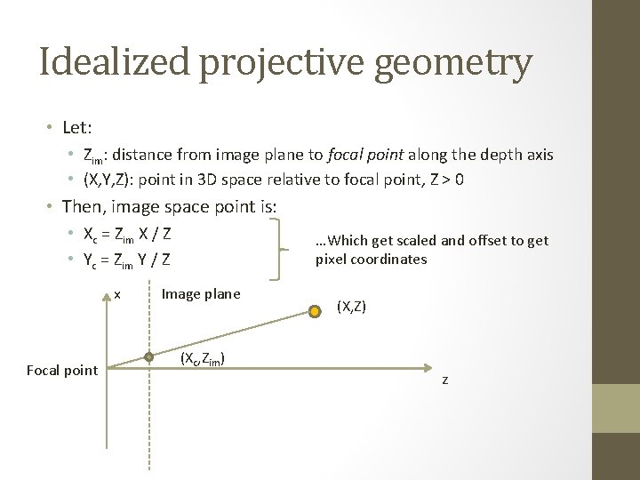
Idealized projective geometry • Let: • Zim: distance from image plane to focal point along the depth axis • (X, Y, Z): point in 3 D space relative to focal point, Z > 0 • Then, image space point is: • Xc = Zim X / Z • Yc = Zim Y / Z x Focal point …Which get scaled and offset to get pixel coordinates Image plane (Xc, Zim) (X, Z) z

Working with Images • On a computer, an image is a 2 D array of sensor values (pixels) • Typically red, green, blue (RGB) channels, though other representations exist (monochrome, CMYK, RGBA, etc) • Quantized, usually each channel => 256 values (8 bits, or 1 byte) • (Compression / decompression, e. g. , JPEG, will be assumed given) • Width w, height h • Typically an image comes “packed” into a contiguous chunk of memory containing w*h*c*2 d bits, where c is the number of channels, d is the bit depth • Pixel (i, j) stored in the c*2 d bits starting at memory location (i*w+j)*c*2 d • Typically, i coordinate goes left->right, j coordinate goes top->bottom

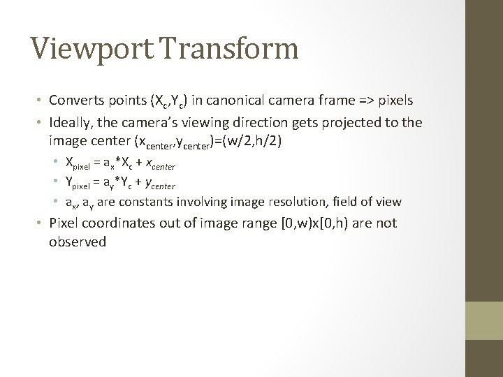
Viewport Transform • Converts points (Xc, Yc) in canonical camera frame => pixels • Ideally, the camera’s viewing direction gets projected to the image center (xcenter, ycenter)=(w/2, h/2) • Xpixel = ax*Xc + xcenter • Ypixel = ay*Yc + ycenter • ax, ay are constants involving image resolution, field of view • Pixel coordinates out of image range [0, w)x[0, h) are not observed

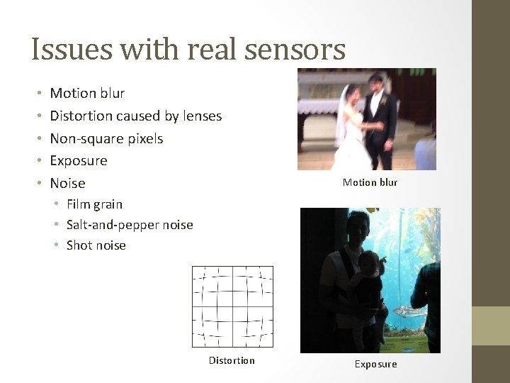
Issues with real sensors • • • Motion blur Distortion caused by lenses Non-square pixels Exposure Noise Motion blur • Film grain • Salt-and-pepper noise • Shot noise Distortion Exposure

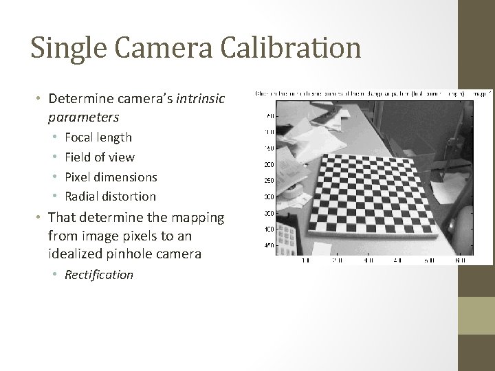
Single Camera Calibration • Determine camera’s intrinsic parameters • • Focal length Field of view Pixel dimensions Radial distortion • That determine the mapping from image pixels to an idealized pinhole camera • Rectification

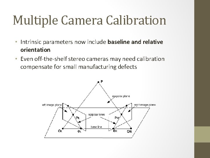
Multiple Camera Calibration • Intrinsic parameters now include baseline and relative orientation • Even off-the-shelf stereo cameras may need calibration compensate for small manufacturing defects

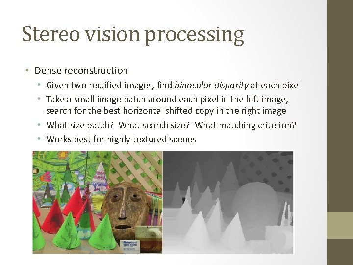
Stereo vision processing • Dense reconstruction • Given two rectified images, find binocular disparity at each pixel • Take a small image patch around each pixel in the left image, search for the best horizontal shifted copy in the right image • What size patch? What search size? What matching criterion? • Works best for highly textured scenes

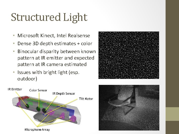
Structured Light • Microsoft Kinect, Intel Realsense • Dense 3 D depth estimates + color • Binocular disparity between known pattern at IR emitter and expected pattern at IR camera estimated • Issues with bright light (esp. outdoor)

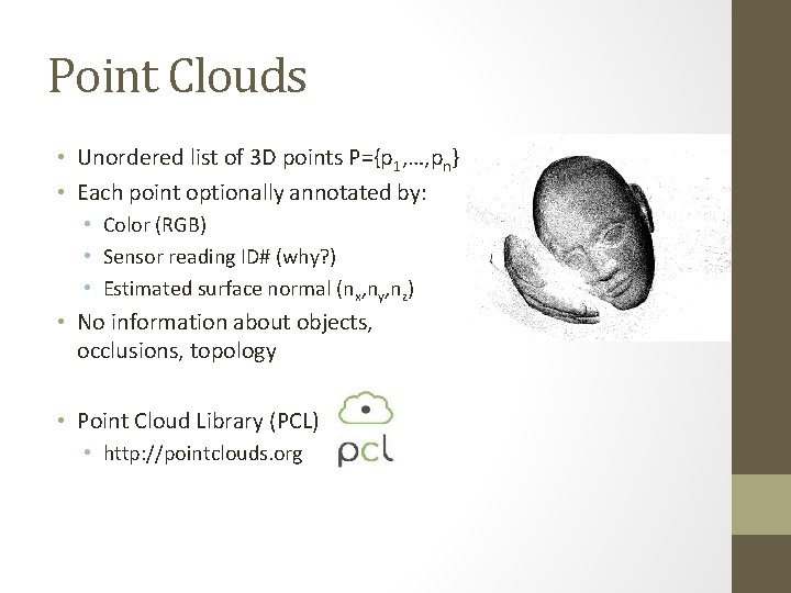
Point Clouds • Unordered list of 3 D points P={p 1, …, pn} • Each point optionally annotated by: • Color (RGB) • Sensor reading ID# (why? ) • Estimated surface normal (nx, ny, nz) • No information about objects, occlusions, topology • Point Cloud Library (PCL) • http: //pointclouds. org

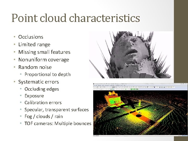
Point cloud characteristics • • • Occlusions Limited range Missing small features Nonuniform coverage Random noise • Proportional to depth • Systematic errors • • • Occluding edges Exposure Calibration errors Specular, transparent surfaces Fog / clouds / rain TOF cameras: Multiple bounces

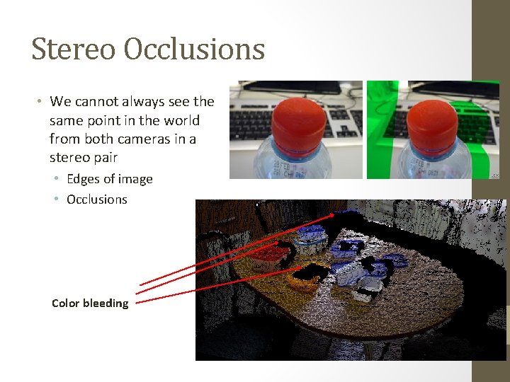
Stereo Occlusions • We cannot always see the same point in the world from both cameras in a stereo pair • Edges of image • Occlusions Color bleeding

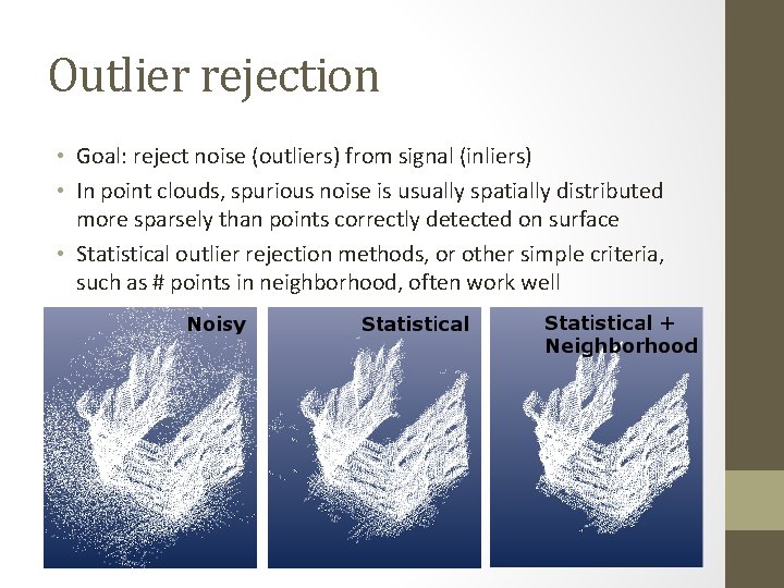
Outlier rejection • Goal: reject noise (outliers) from signal (inliers) • In point clouds, spurious noise is usually spatially distributed more sparsely than points correctly detected on surface • Statistical outlier rejection methods, or other simple criteria, such as # points in neighborhood, often work well

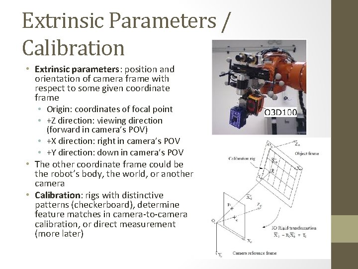
Extrinsic Parameters / Calibration • Extrinsic parameters: position and orientation of camera frame with respect to some given coordinate frame • Origin: coordinates of focal point • +Z direction: viewing direction (forward in camera’s POV) • +X direction: right in camera’s POV • +Y direction: down in camera’s POV • The other coordinate frame could be the robot’s body, the world, or another camera • Calibration: rigs with distinctive patterns (checkerboard), determine feature matches in camera-to-camera calibration, or direct measurement (more later)

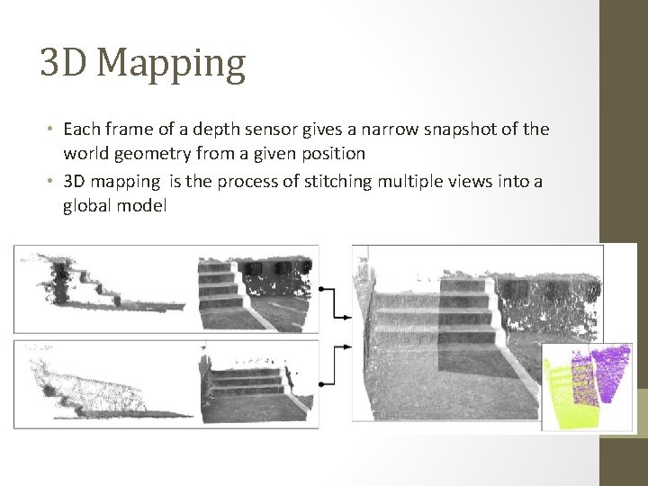
3 D Mapping • Each frame of a depth sensor gives a narrow snapshot of the world geometry from a given position • 3 D mapping is the process of stitching multiple views into a global model

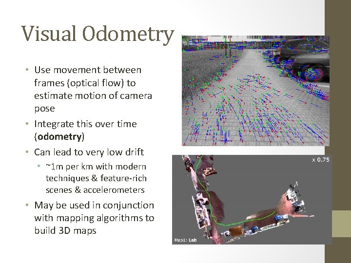
Visual Odometry • Use movement between frames (optical flow) to estimate motion of camera pose • Integrate this over time (odometry) • Can lead to very low drift • ~1 m per km with modern techniques & feature-rich scenes & accelerometers • May be used in conjunction with mapping algorithms to build 3 D maps

Next week • 3 D mapping • CVAA Ch 12. 2