Dynamic Planning Optimal Control ECE 383 ME 442

, avoid modeling dynamics (ex: PID")

 • Today • • • Principles Ch 7. 2 Concept of")
 • Idea: repeatedly compute feedforward control using model of the")


")


")


![Lie Bracket [X, Y] = d. Y. X – d. X. Y X 1/](https://slidetodoc.com/presentation_image/41000a1a1fef95ae7919d0f8f9184f01/image-28.jpg "Lie Bracket [X, Y] = d. Y. X – d. X. Y X 1/")


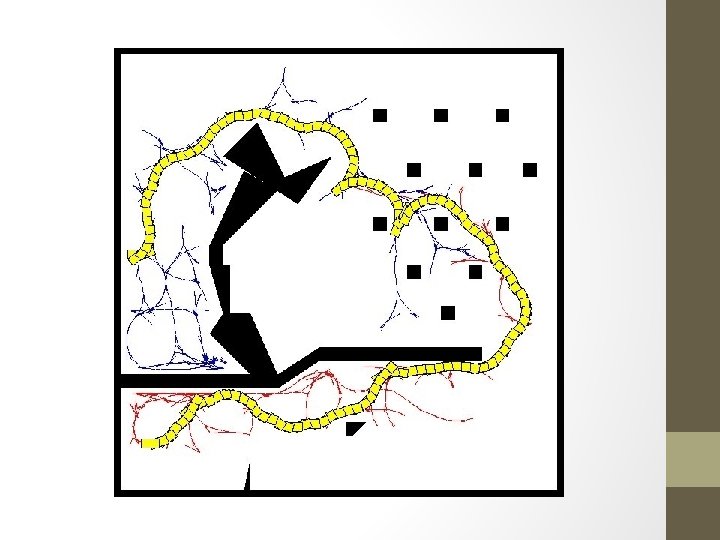
![Lie Bracket Maneuvers • Problem: To move distance d along vector field U=[X, Y]](https://slidetodoc.com/presentation_image/41000a1a1fef95ae7919d0f8f9184f01/image-32.jpg "Lie Bracket Maneuvers • Problem: To move distance d along vector field U=[X, Y]")
 h h q r dq (x, y,")


 tan f")


 • Build a tree T of configurations")


- Slides: 51
Dynamic Planning / Optimal Control ECE 383 / ME 442
Context: Model-based control 1. Model-free control: choose u(x, t), avoid modeling dynamics (ex: PID control) • Good for simple problems • Low computational complexity • Requires parameter tuning • Difficult to choose suitable policy for complex systems • Has no performance guarantees 2. Model-based control: model dynamics and choose u to yield a “good” future trajectory. (ex: gravity compensation, optimal control) • Able to achieve better performance (e. g. , optimality) • Dynamics may be hard to model • Must usually be combined with model-free control or model adaptation to compensate for un-modeled errors (implementation difficulty)
Context: Myopic vs Predictive •
Agenda (2 day) • Today • • • Principles Ch 7. 2 Concept of model predictive control Controllability Kinematic reductions & maneuvers in motion planning Sampling-based planning with dynamics • Next time • • Principles Ch 8 Optimal control Trajectory optimization Bellman equation
Model predictive control (MPC) • Idea: repeatedly compute feedforward control using model of the dynamics, prediction • In other words, rapid replanning Feedforward calculation u=uff Plant xdes x(t)
Kinematic Planning • So far, all constraints on motion have been represented as C-space obstacles • Dynamic constraints: omnidirectional motion in Cspace not permitted
Kinematic reductions • Can we plan kinematically-feasible paths and then convert them to dynamically-feasible ones? • Sometimes • Kinematic reduction
Holonomic systems • Omnidirectional mobile base: holonomic Differential drive: non-holonomic
Planning for Holonomic Systems = Kinematic planning • Most interesting dynamic systems are nonholonomic… but maybe we can do this approximately
Sea horses By: Saya h.
Path Deformation Holonomic path Nonholonomic path
Example: 1 D Point Mass x v v dx/dt = dv dv/dt = f / M |f|<=fmax Solution: v(t) = v(0)+t f /M x(t) = x(0)+t v(0) + ½ t 2 f / M x
Example: Car-Like Robot dx/dt = v cosq dy/dt = v sinq f y q dq/dt = (v/L) tan f q f L dx sinq – dy cosq = 0 |f| < F x Configuration space is 3 -dimensional: q = (x, y, q) But control space is 2 -dimensional: (v, f) with |v| = sqrt[(dx/dt)2+(dy/dt)2]
Example: Car-Like Robot dx/dt = v cosq dy/dt = v sinq f L q y dx sinq – dy cosq = 0 dq/dt = (v/L) tan f q |f| < F f x q = (x, y, q) q’= dq/dt = (dx/dt, dy/dt, dq/dt) dx sinq – dy cosq = 0 is a particular form of f(q, q’)=0 A robot is nonholonomic if its motion is constrained by a nonintegrable equation of the form f(q, q’) = 0
Example: Car-Like Robot dx/dt = v cosq dy/dt = v sinq f L q y dx sinq – dy cosq = 0 dq/dt = (v/L) tan f q |f| < F f x Lower-bounded turning radius
How Can This Work? Tangent Space/Velocity Space f L q y q (x, y, q) q (dx, dy, dq) f x dx/dt = v cosq dy/dt = v sinq dq/dt = (v/L) tan f |f| < F (dx, dy) x q y
How Can This Work? Tangent Space/Velocity Space f L q y q (x, y, q) q (dx, dy, dq) f x dx/dt = v cosq dy/dt = v sinq dq/dt = (v/L) tan f |f| < F (dx, dy) x q y
Kinematic Reduction of 1 D Point Mass • If: • Constraints are time-invariant • Starts and stops at rest • Then we only need to consider position x 1+e 1. Speed up 2. Slow down
Dynamic Execution of Kinematic Paths • For fully actuated N-D robots, a collision-free path can be executed “slowly enough” v x
Optimal Straight-line Following • Given a particle with velocity and acceleration bounds, what is the optimal motion between two points, starting and stopping at rest?
Optimal Straight-line Following • Given a particle with velocity and acceleration bounds, what is the optimal motion between two points, starting and stopping at rest? • Max acceleration, (optional) max velocity, max deceleration x v+ a- a+ t • Trapezoidal velocity profile v vmax t
Optimization of Dynamic Paths for Robot Arms Hauser and Ng Thow Hing (2010)
Small-Time Local Controllability • A system is small-time locally controllable if at a given configuration q, it can reach an open neighborhood of q with “small” motions e q SLTC Not SLTC
Small-Time Local Controllability • A system is small-time locally controllable if at a given configuration q, it can reach an open neighborhood of q with “small” motions • Surprise: simple car model is STLC e q SLTC Not SLTC
Lie Bracket Maneuver made of 4 motions -X -Y Y X (dt)
Lie Bracket Maneuver made of 4 motions For example: dx/dt = v cosq dy/dt = v sinq X: Going straight T dq/dt = (v/L) tan f Y: Turning, angle f T |f| < F
Lie Bracket Maneuver made of 4 motions For example: -X X: Going straight -Y T Y: Turning, angle f T [X, Y] (dt 2 ) Lie bracket Y X (dt)
Lie Bracket [X, Y] = d. Y. X – d. X. Y X 1/ x X 1/ y X 1/ q d. X = X 2/ x X 2/ y X 2/ q X 3/ x X 3/ y X 3/ q [X, Y] Lin(X, Y) the motion constraint is nonholonomic -X -Y [X, Y] (dt 2 ) Lie bracket Y X (dt)
Lie Bracket d. X = 0 0 -v sin θ 0 0 v cos θ 0 0 0 d. Y = 0 0 -v sin θ 0 0 v cos θ 0 0 0 -X X: Going straight -Y T Y: Turning, angle f T [X, Y] = d. Y. X – d. X. Y = 0 0 0 [X, Y] (dt 2 ) Y X (dt) v 2/L sin θ tan φ -v 2/L cos θ tan φ 0
Sufficient condition for STLC 1. Let S = {Xi}, i=1, …, k be control vector fields over n dimensional manifold 2. For each pair Xi, Xj in S: • Compute lie bracket U = [Xi, Xj] • If U Lin(S), then add U to S and repeat step 2 3. If |S|=n, then STLC
Tractor-Trailer Example • 4 -D configuration space • 2 -D control/velocity space • two independent velocity vectors X and Y • U = [X, Y] Lin(X, Y) • V = [X, U] Lin(X, Y, U)
Lie Bracket Maneuvers • Problem: To move distance d along vector field U=[X, Y] using Lie bracket, may need to move much farther in C-space • Solution: Use better maneuvers
Type 1 Maneuver CYL(x, y, dq, h) h h q r dq (x, y, q) dq (x, y) dq r h= 2 r tandq d = 2 r(1/cosdq - 1) > 0 When dq 0, so does d and the cylinder becomes arbitrarily small Allows sideways motion
Type 2 Maneuver Allows pure rotation
Combination
Coverage of a Path by Cylinders q q q’+ y x
Path Examples
Drawbacks of Two-phase Planning • Final path can be far from optimal • Not applicable to robots that are not locally controllable (e. g. , car that can only move forward)
Reeds and Shepp Paths
Reeds and Shepp Paths CC|C 0 CC|C C|CS 0 C|C Given any two configurations, the shortest RS paths between them is also the shortest path
Example of Generated Path Holonomic Nonholonomic
Path Optimization
Perspective • If one can determine kinematic reductions or steering functions, usually the best method is to reduce to kinematic planning + postprocessing • If these cannot be found, must resort to the approach of control-based planning in state space
Control-Based Sampling § § PRM sampling technique: Pick each milestone in some region Control-based sampling: 1. 2. 3. Pick control vector (at random or not) Integrate equation of motion over short duration (picked at random or not) If the motion is collision-free, then the endpoint is the new milestone Tree-structured roadmaps Need for endgame regions
Example dx/dt = v cosq dy/dt = v sinq dq/dt = (v/L) tan f |f| < F 1. Select a milestone m 2. Pick v, f, and dt 3. Integrate motion from m new milestone m’
Example Indexing array: A 3 -D grid is placed over the configuration space. Each milestone falls into one cell of the grid. A maximum number of milestones is allowed in each cell (e. g. , 2 or 3). Asymptotic completeness: If a path exists, the planner is guaranteed to find one if the resolution of the grid is fine enough.
Computed Paths Car That Can Only Turn Left Tractor-trailer jmax=45 o, jmin=22. 5 o jmax=45 o
Control-Sampling RRT • Configuration generator f(x, u) • Build a tree T of configurations • Extend: • Sample a configuration xrand from X at random • Find the node xnear in T that is closest to xrand • Pick a control u that brings f(xnear, u) close to xrand • Add f(xnear, u) as a child of xnear in T
Weaknesses of RRT’s strategy • Depends on the domain from which xrand is sampled (sampling strategy) • Depends on the notion of “closest” (metric sensitivity) • A tree that is grown “badly” by accident can greatly slow convergence (history dependence)
Next time • Considering optimality • Principles Ch 8