Introduction to Control ECE 383 ME 442 Fall

Introduction to Control ECE 383 / ME 442 Fall 2015 Kris Hauser

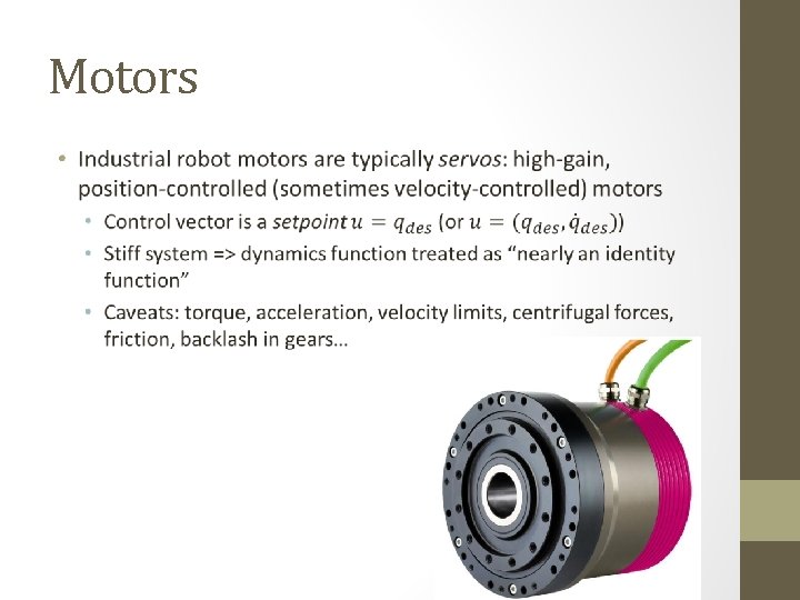
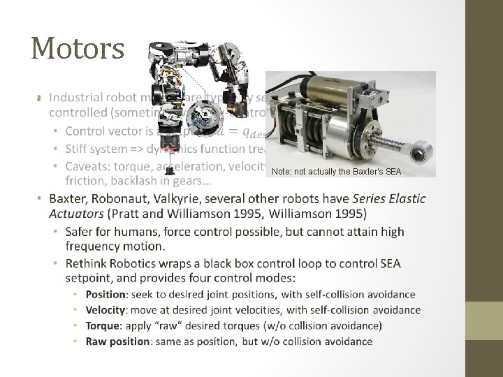
Motors •

Motors • Note: not actually the Baxter’s SEA

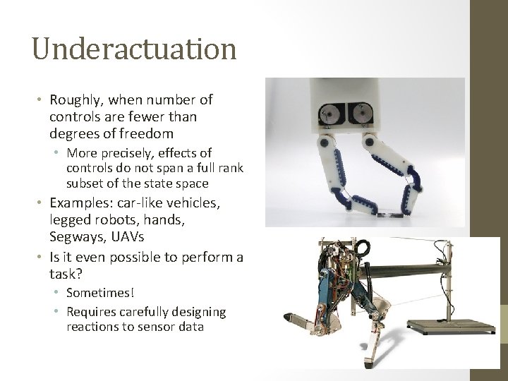
Underactuation • Roughly, when number of controls are fewer than degrees of freedom • More precisely, effects of controls do not span a full rank subset of the state space • Examples: car-like vehicles, legged robots, hands, Segways, UAVs • Is it even possible to perform a task? • Sometimes! • Requires carefully designing reactions to sensor data

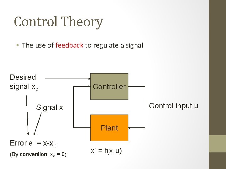
Control Theory • The use of feedback to regulate a signal Desired signal xd Controller Control input u Signal x Plant Error e = x-xd (By convention, xd = 0) x’ = f(x, u)

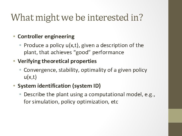
What might we be interested in? • Controller engineering • Produce a policy u(x, t), given a description of the plant, that achieves “good” performance • Verifying theoretical properties • Convergence, stability, optimality of a given policy u(x, t) • System identification (system ID) • Describe the plant using a computational model, e. g. , for simulation, policy optimization, etc

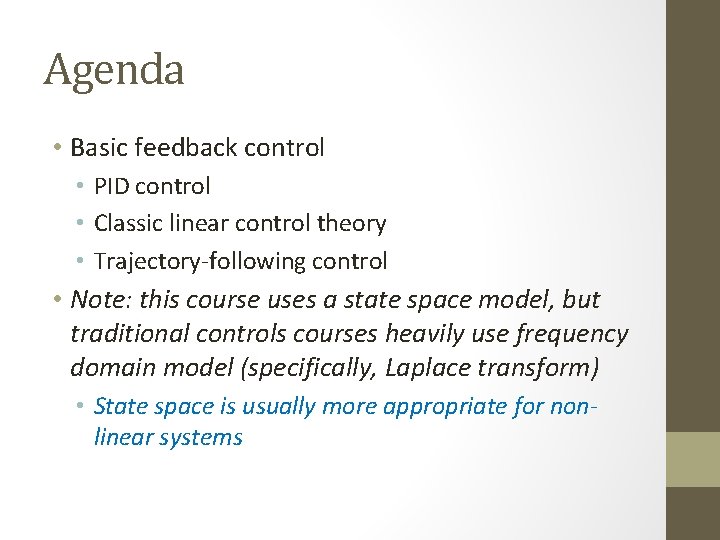
Agenda • Basic feedback control • PID control • Classic linear control theory • Trajectory-following control • Note: this course uses a state space model, but traditional controls courses heavily use frequency domain model (specifically, Laplace transform) • State space is usually more appropriate for nonlinear systems

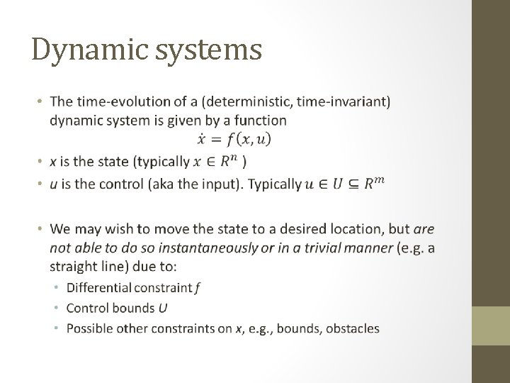
Dynamic systems •

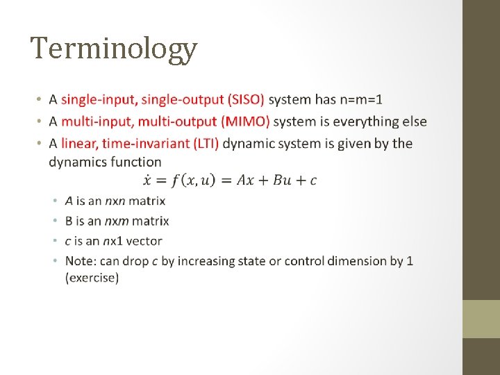
Terminology •

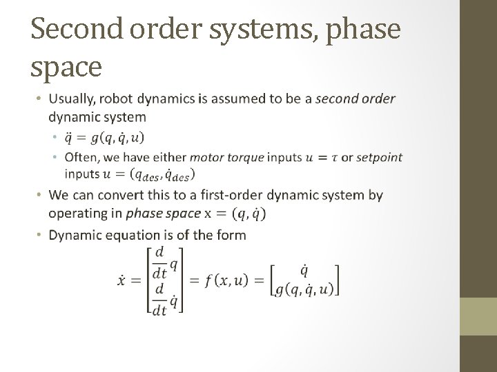
Second order systems, phase space •

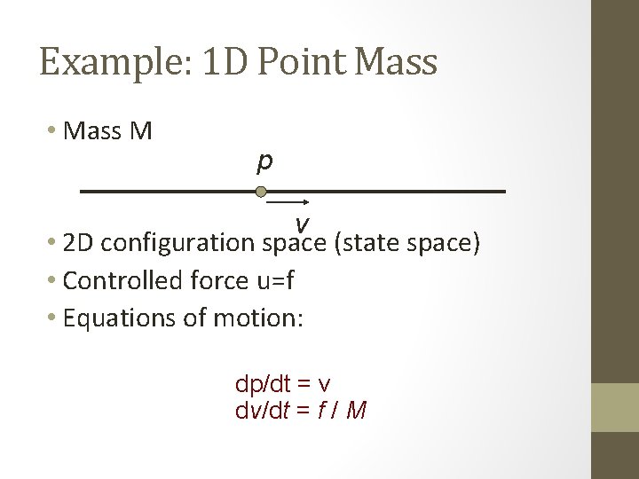
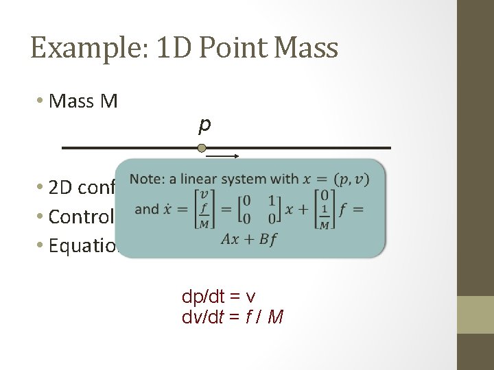
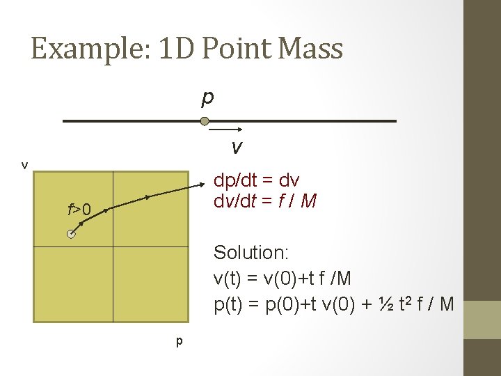
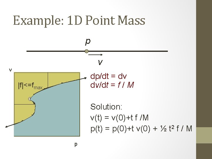
Example: 1 D Point Mass • Mass M p v • 2 D configuration space (state space) • Controlled force u=f • Equations of motion: dp/dt = v dv/dt = f / M

Example: 1 D Point Mass • Mass M p v • 2 D configuration space (state space) • Controlled force u=f • Equations of motion: dp/dt = v dv/dt = f / M

Example: 1 D Point Mass p v v dp/dt = dv dv/dt = f / M f=0 Solution: v(t) = v(0)+t f /M p(t) = p(0)+t v(0) + ½ t 2 f / M p

Example: 1 D Point Mass p v v dp/dt = dv dv/dt = f / M f>0 Solution: v(t) = v(0)+t f /M p(t) = p(0)+t v(0) + ½ t 2 f / M p

Example: 1 D Point Mass p v v dp/dt = dv dv/dt = f / M f<0 Solution: v(t) = v(0)+t f /M p(t) = p(0)+t v(0) + ½ t 2 f / M p

Example: 1 D Point Mass p v v dp/dt = dv dv/dt = f / M |f|<=fmax Solution: v(t) = v(0)+t f /M p(t) = p(0)+t v(0) + ½ t 2 f / M p

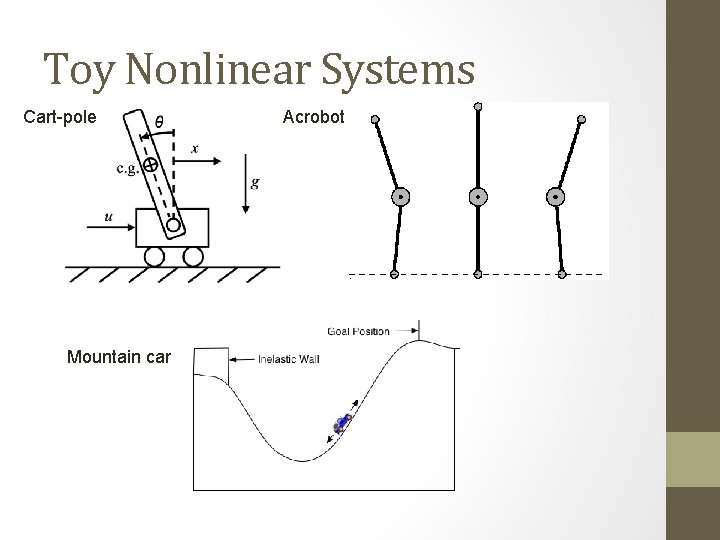
Toy Nonlinear Systems Cart-pole Mountain car Acrobot

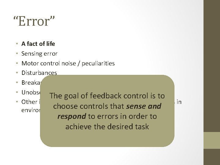
“Error” • • A fact of life Sensing error Motor control noise / peculiarities Disturbances Breakages Unobservables Other intelligent agents (e. g. , human operators, humans in environment)

“Error” • • A fact of life Sensing error Motor control noise / peculiarities Disturbances Breakages Unobservables The goal of feedback control is to Other intelligent agents (e. g. , human operators, humans in choose controls that sense and environment) respond to errors in order to achieve the desired task

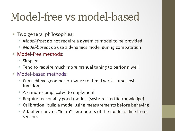
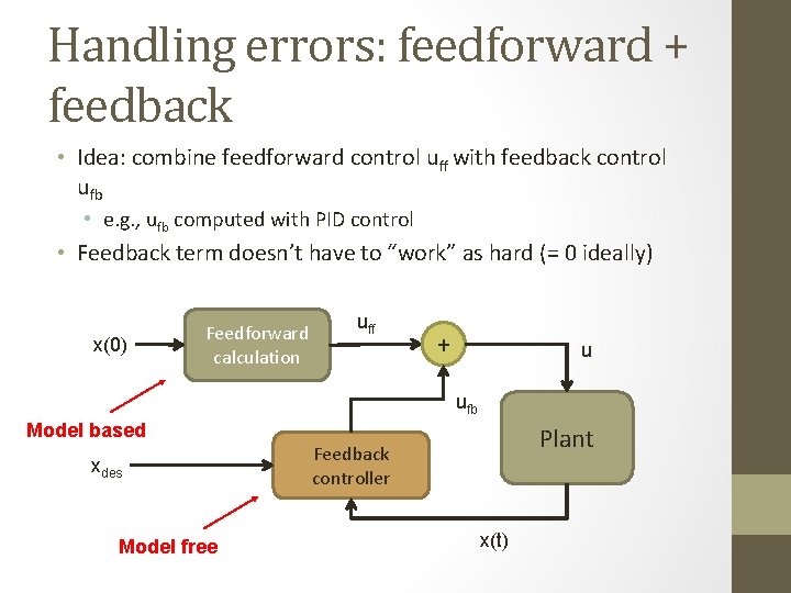
Model-free vs model-based • Two general philosophies: • Model-free: do not require a dynamics model to be provided • Model-based: do use a dynamics model during computation • Model-free methods: • Simpler • Tend to require much more manual tuning to perform well • Model-based methods: • Can achieve good performance (optimal w. r. t. some cost function) • Are more complicated to implement • Require reasonably good models (system-specific knowledge) • Calibration: build a model using measurements before behaving • Adaptive control: “learn” parameters of the model online from sensors

PID control • Proportional-Integral-Derivative controller • A workhorse of 1 D control systems • Model-free, myopic

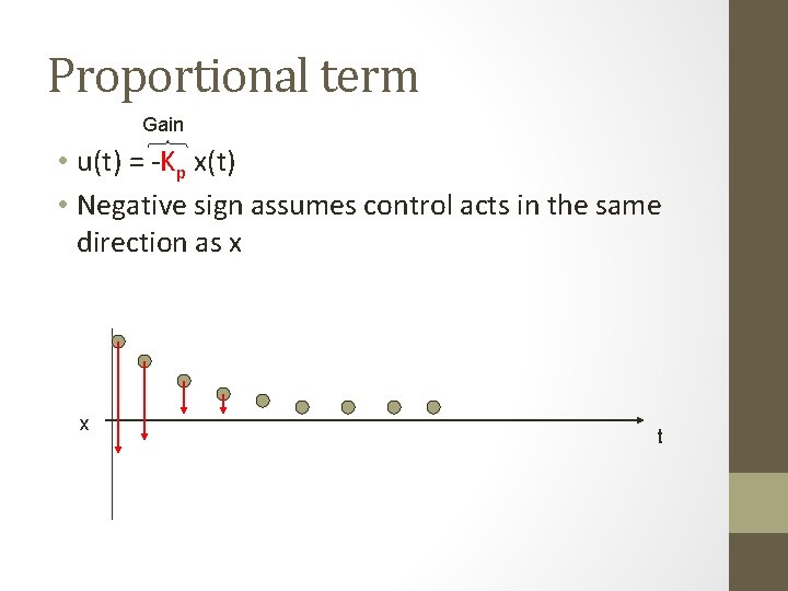
Proportional term Gain • u(t) = -Kp x(t) • Negative sign assumes control acts in the same direction as x x t

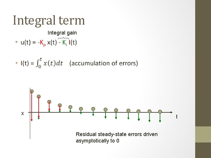
Integral term Integral gain • x t Residual steady-state errors driven asymptotically to 0

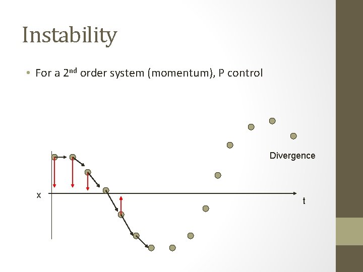
Instability • For a 2 nd order system (momentum), P control Divergence x t

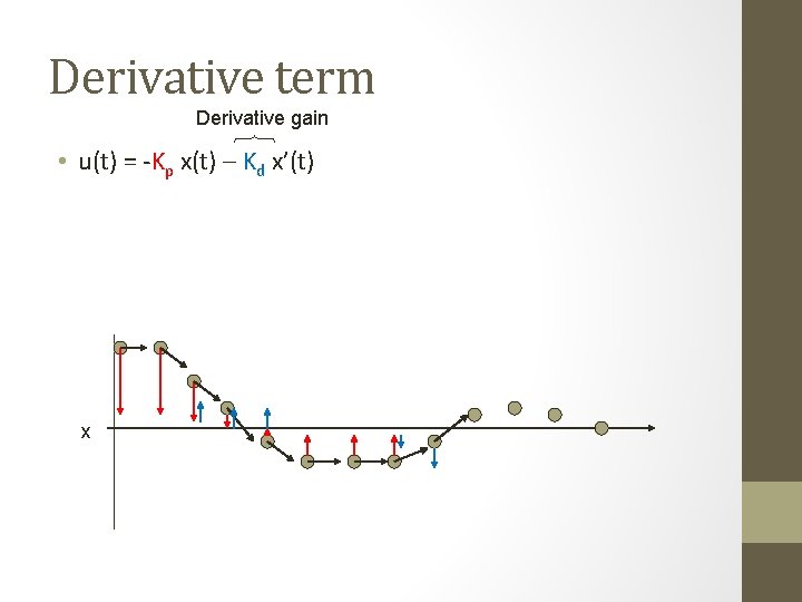
Derivative term Derivative gain • u(t) = -Kp x(t) – Kd x’(t) x

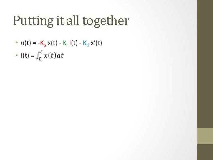
Putting it all together •

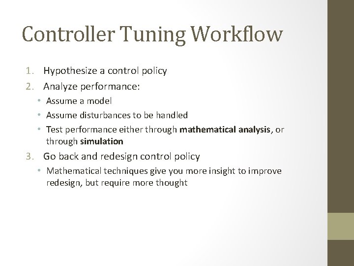
Controller Tuning Workflow 1. Hypothesize a control policy 2. Analyze performance: • Assume a model • Assume disturbances to be handled • Test performance either through mathematical analysis, or through simulation 3. Go back and redesign control policy • Mathematical techniques give you more insight to improve redesign, but require more thought

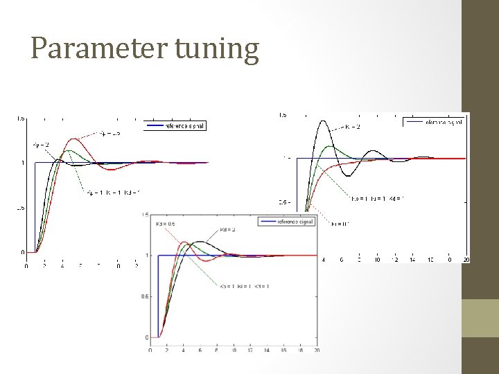
Parameter tuning

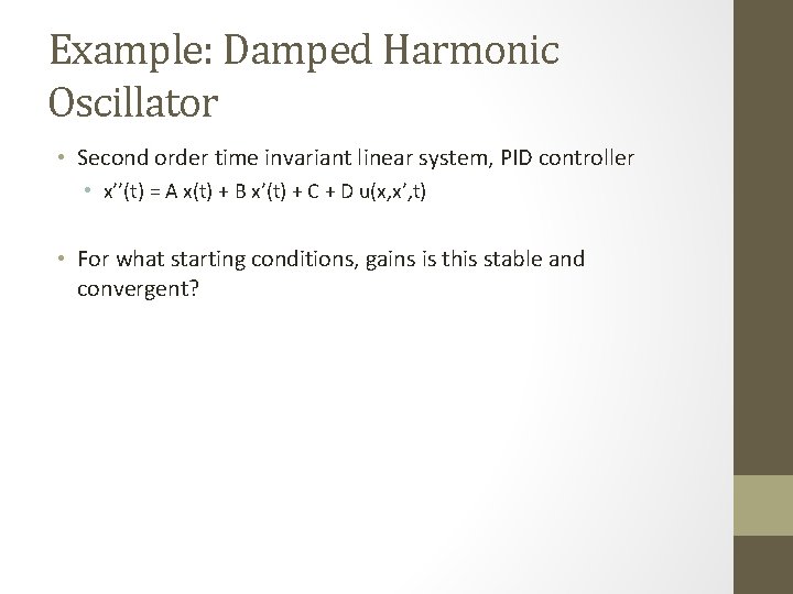
Example: Damped Harmonic Oscillator • Second order time invariant linear system, PID controller • x’’(t) = A x(t) + B x’(t) + C + D u(x, x’, t) • For what starting conditions, gains is this stable and convergent?

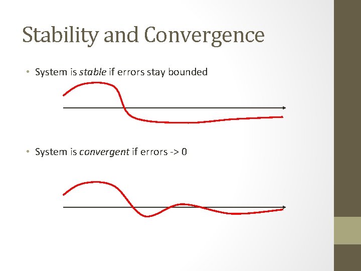
Stability and Convergence • System is stable if errors stay bounded • System is convergent if errors -> 0

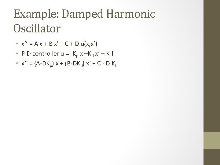
Example: Damped Harmonic Oscillator • x’’ = A x + B x’ + C + D u(x, x’) • PID controller u = -Kp x –Kd x’ – Ki I • x’’ = (A-DKp) x + (B-DKd) x’ + C - D Ki I

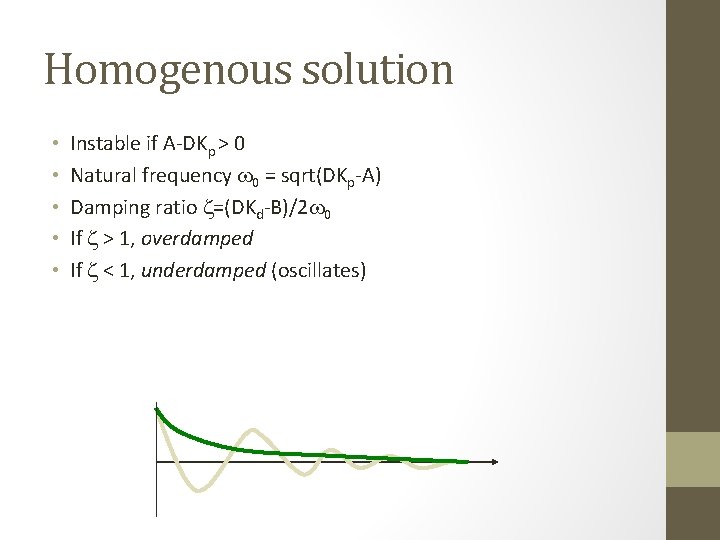
Homogenous solution • • • Instable if A-DKp > 0 Natural frequency w 0 = sqrt(DKp-A) Damping ratio z=(DKd-B)/2 w 0 If z > 1, overdamped If z < 1, underdamped (oscillates)

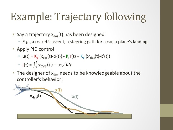
Example: Trajectory following • x(t) xdes(t) x(t)

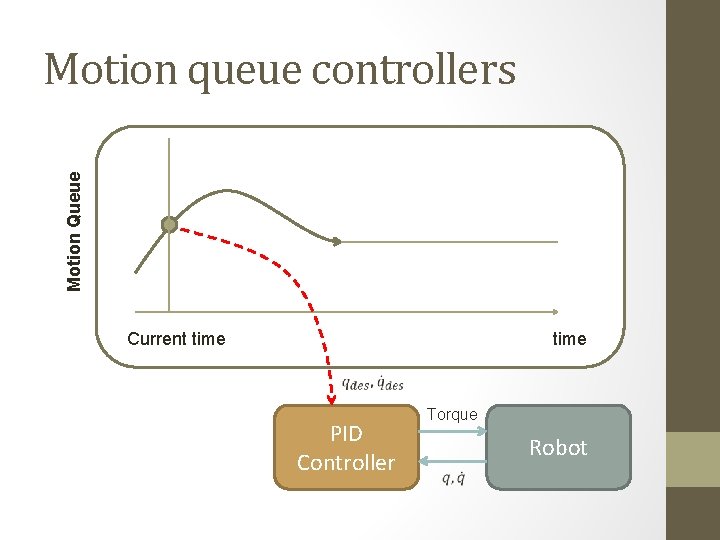
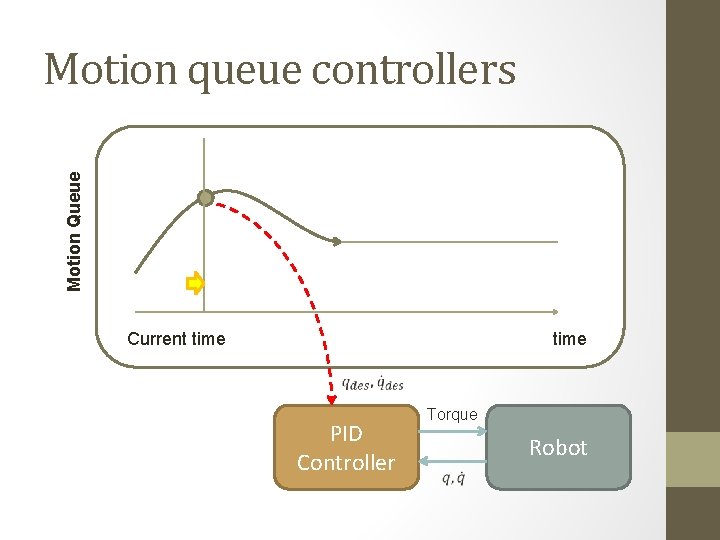
Motion Queue Motion queue controllers Current time PID Controller Torque Robot

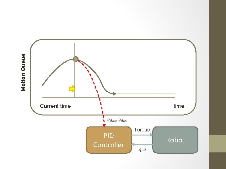
Motion Queue Motion queue controllers Current time PID Controller Torque Robot

Motion Queue Motion queue controllers Current time PID Controller Torque Robot

Parameters: Trajectory suffix y(t): [0, T]->R Motion Queue Append trajectory Current time PID Controller Torque Robot

Motion Queue Current time PID Controller Torque Robot

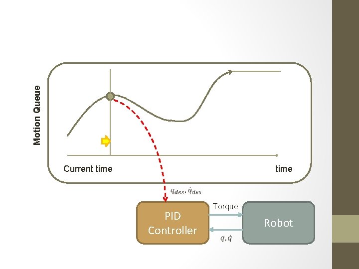
Parameters: Insertion time tinsert Trajectory suffix y(t): [0, T]->R Motion Queue Insert trajectory Current time PID Controller Torque Robot

Motion Queue Current time PID Controller Torque Robot

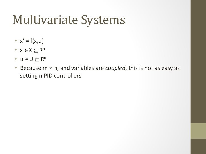
Multivariate Systems • • x’ = f(x, u) x X Rn u U Rm Because m n, and variables are coupled, this is not as easy as setting n PID controllers

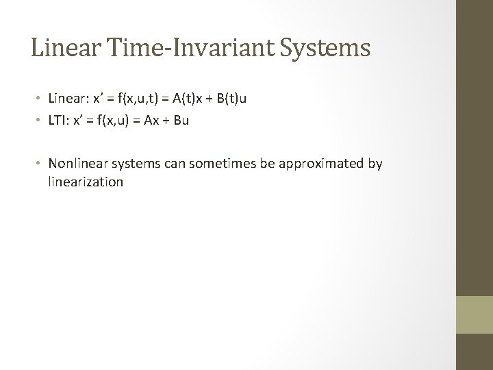
Linear Time-Invariant Systems • Linear: x’ = f(x, u, t) = A(t)x + B(t)u • LTI: x’ = f(x, u) = Ax + Bu • Nonlinear systems can sometimes be approximated by linearization

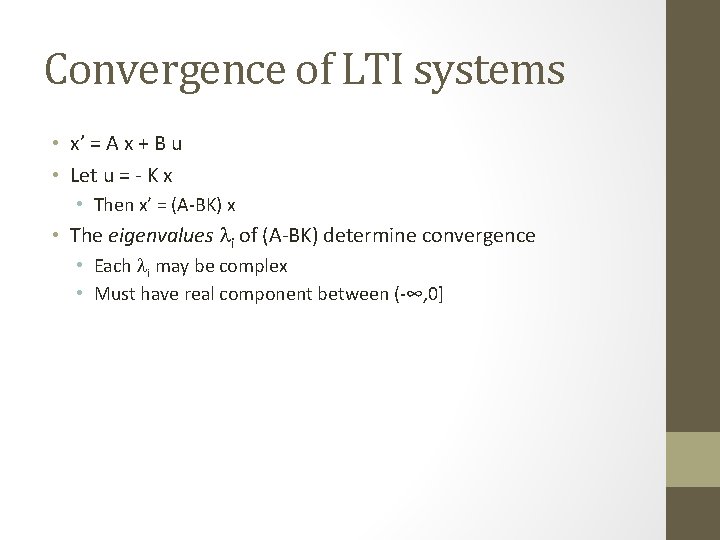
Convergence of LTI systems • x’ = A x + B u • Let u = - K x • Then x’ = (A-BK) x • The eigenvalues li of (A-BK) determine convergence • Each li may be complex • Must have real component between (-∞, 0]

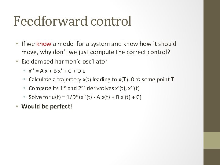
Feedforward control • If we know a model for a system and know how it should move, why don’t we just compute the correct control? • Ex: damped harmonic oscillator • • x’’ = A x + B x’ + C + D u Calculate a trajectory x(t) leading to x(T)=0 at some point T Compute its 1 st and 2 nd derivatives x’(t), x’’(t) Solve for u(t) = 1/D*(x’’(t) - A x(t) + B x’(t) + C) • Would be perfect!

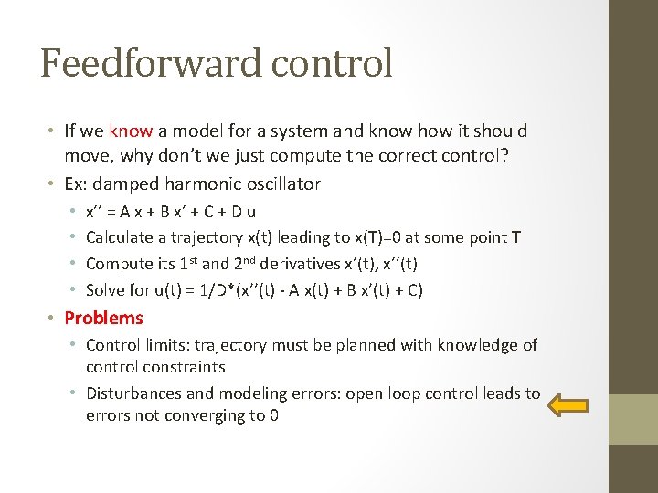
Feedforward control • If we know a model for a system and know how it should move, why don’t we just compute the correct control? • Ex: damped harmonic oscillator • • x’’ = A x + B x’ + C + D u Calculate a trajectory x(t) leading to x(T)=0 at some point T Compute its 1 st and 2 nd derivatives x’(t), x’’(t) Solve for u(t) = 1/D*(x’’(t) - A x(t) + B x’(t) + C) • Problems • Control limits: trajectory must be planned with knowledge of control constraints • Disturbances and modeling errors: open loop control leads to errors not converging to 0

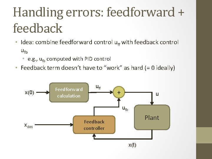
Handling errors: feedforward + feedback • Idea: combine feedforward control uff with feedback control ufb • e. g. , ufb computed with PID control • Feedback term doesn’t have to “work” as hard (= 0 ideally) x(0) Feedforward calculation uff + u ufb xdes Plant Feedback controller x(t)

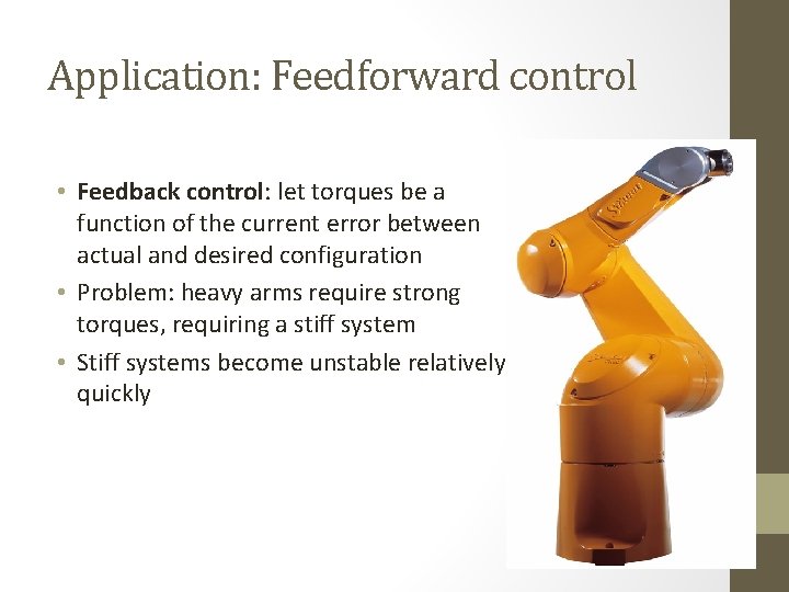
Application: Feedforward control • Feedback control: let torques be a function of the current error between actual and desired configuration • Problem: heavy arms require strong torques, requiring a stiff system • Stiff systems become unstable relatively quickly

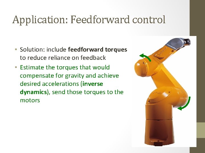
Application: Feedforward control • Solution: include feedforward torques to reduce reliance on feedback • Estimate the torques that would compensate for gravity and achieve desired accelerations (inverse dynamics), send those torques to the motors

Handling errors: feedforward + feedback • Idea: combine feedforward control uff with feedback control ufb • e. g. , ufb computed with PID control • Feedback term doesn’t have to “work” as hard (= 0 ideally) x(0) Feedforward calculation uff + u ufb Model based xdes Model free Plant Feedback controller x(t)

Next class: Klamp’t simulation and control • Reading: • Klamp’t simulation tutorial