Utilizing AICD and GIMIC programs to study magnetically

Utilizing AICD and GIMIC programs to study magnetically induced current density Sobereva 2012 -Jul-26

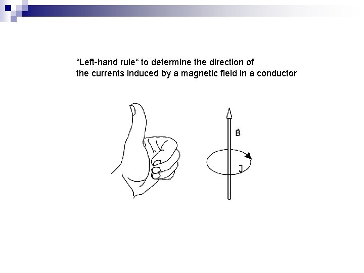
“Left-hand rule“ to determine the direction of the currents induced by a magnetic field in a conductor

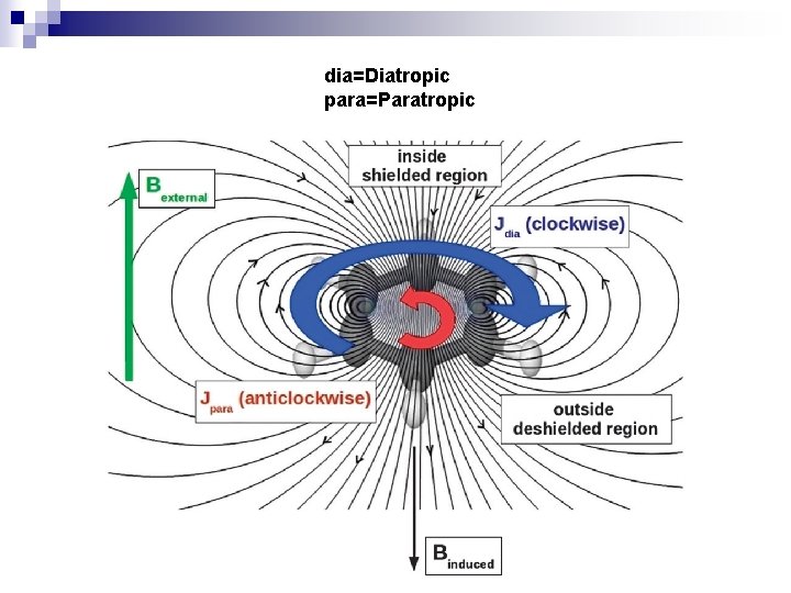
dia=Diatropic para=Paratropic

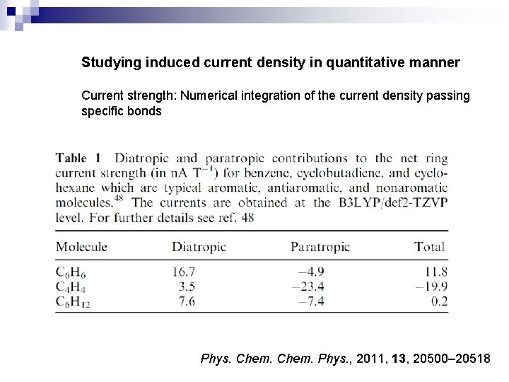
l. Aromatic molecules: The diatropic component on the outside of the molecules dominates over the paratropic one inside the ring yielding a net diatropic current l. Antiaromatic molecules: The paratropic current inside the ring dominates l. Nonaromatic molecules: Also sustain diatropic and paratropic ring currents, but the two components cancel, yielding a minuscule net current

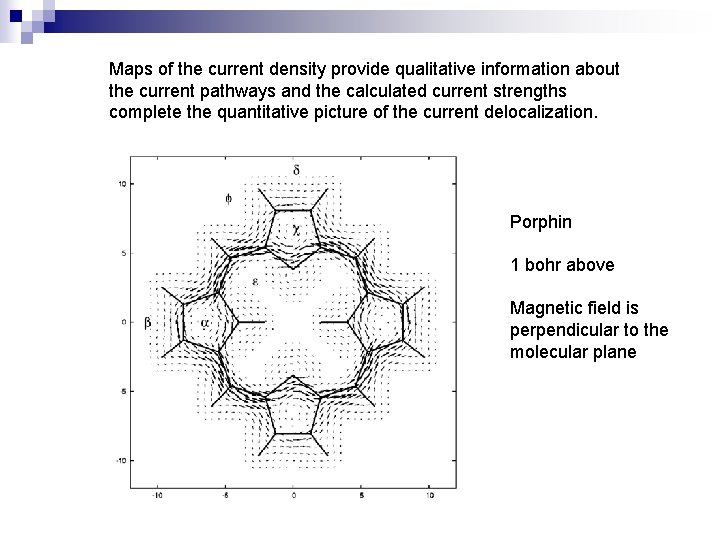
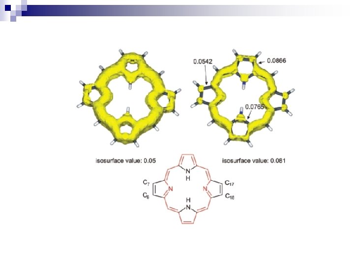
Maps of the current density provide qualitative information about the current pathways and the calculated current strengths complete the quantitative picture of the current delocalization. Porphin 1 bohr above Magnetic field is perpendicular to the molecular plane

Studying induced current density in quantitative manner Current strength: Numerical integration of the current density passing specific bonds Phys. Chem. Phys. , 2011, 13, 20500– 20518

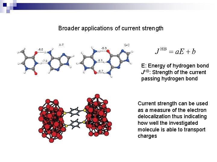
Broader applications of current strength E: Energy of hydrogen bond JHB: Strength of the current passing hydrogen bond Current strength can be used as a measure of the electron delocalization thus indicating how well the investigated molecule is able to transport charges

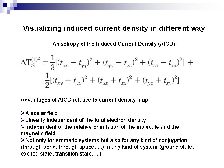
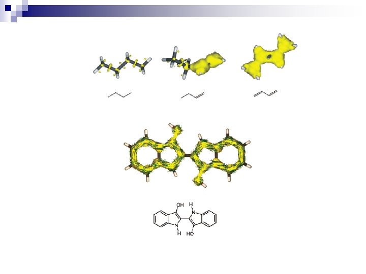
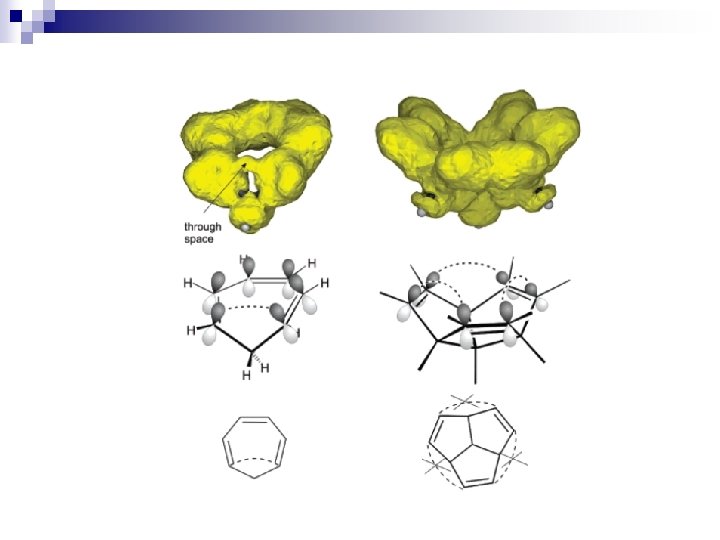
Visualizing induced current density in different way Anisotropy of the Induced Current Density (AICD) Advantages of AICD relative to current density map ØA scalar field ØLinearly independent of the total electron density ØIndependent of the relative orientation of the molecule and the magnetic field ØNot only for aromatic systems but also for any kind of conjugation (through bond, through space, . . . ) in any kind of system (ground state, excited state, transition state, . . . )

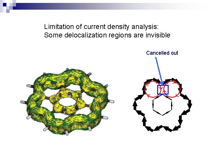
Limitation of current density analysis: Some delocalization regions are invisible Cancelled out

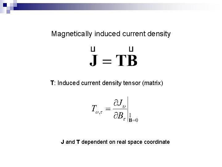
Magnetically induced current density T: Induced current density tensor (matrix) J and T dependent on real space coordinate

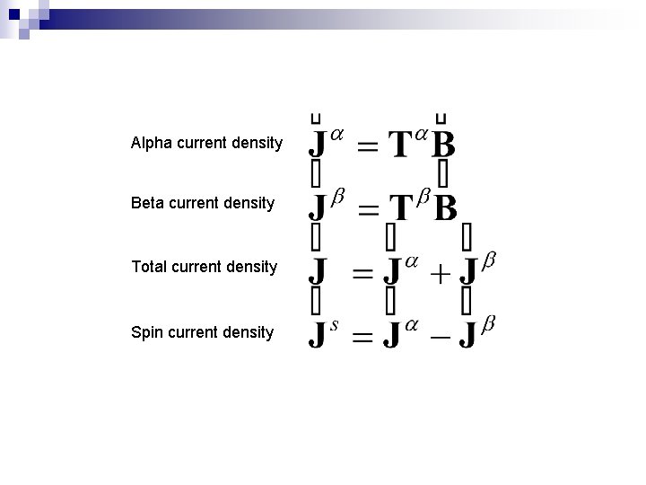
Alpha current density Beta current density Total current density Spin current density

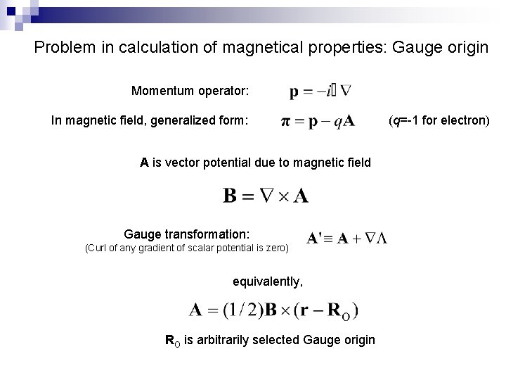
Problem in calculation of magnetical properties: Gauge origin Momentum operator: In magnetic field, generalized form: A is vector potential due to magnetic field Gauge transformation: (Curl of any gradient of scalar potential is zero) equivalently, RO is arbitrarily selected Gauge origin (q=-1 for electron)

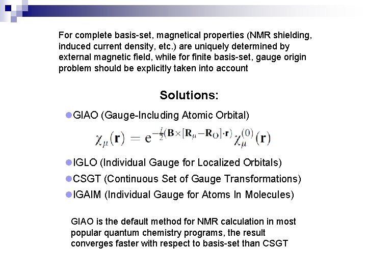
For complete basis-set, magnetical properties (NMR shielding, induced current density, etc. ) are uniquely determined by external magnetic field, while for finite basis-set, gauge origin problem should be explicitly taken into account Solutions: l. GIAO (Gauge-Including Atomic Orbital) l. IGLO (Individual Gauge for Localized Orbitals) l. CSGT (Continuous Set of Gauge Transformations) l. IGAIM (Individual Gauge for Atoms In Molecules) GIAO is the default method for NMR calculation in most popular quantum chemistry programs, the result converges faster with respect to basis-set than CSGT

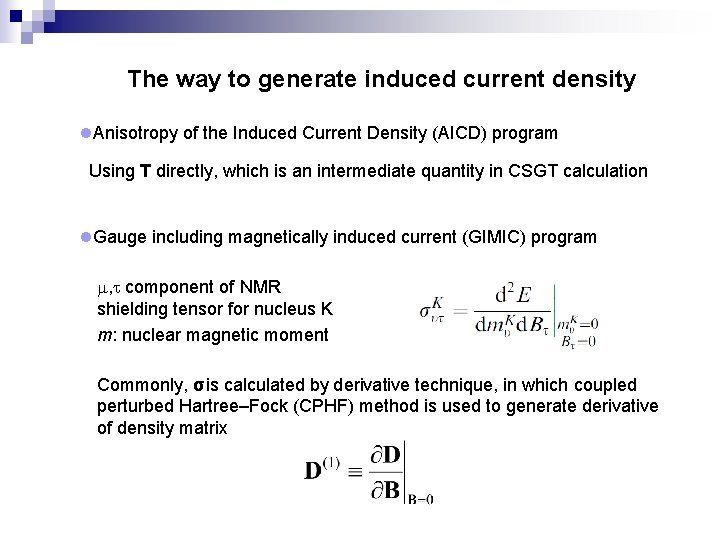
The way to generate induced current density l. Anisotropy of the Induced Current Density (AICD) program Using T directly, which is an intermediate quantity in CSGT calculation l. Gauge including magnetically induced current (GIMIC) program , component of NMR shielding tensor for nucleus K m: nuclear magnetic moment Commonly, σis calculated by derivative technique, in which coupled perturbed Hartree–Fock (CPHF) method is used to generate derivative of density matrix

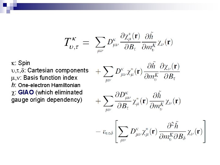
: Spin , , : Cartesian components , : Basis function index h: One-electron Hamiltonian : GIAO (which eliminated gauge origin dependency)

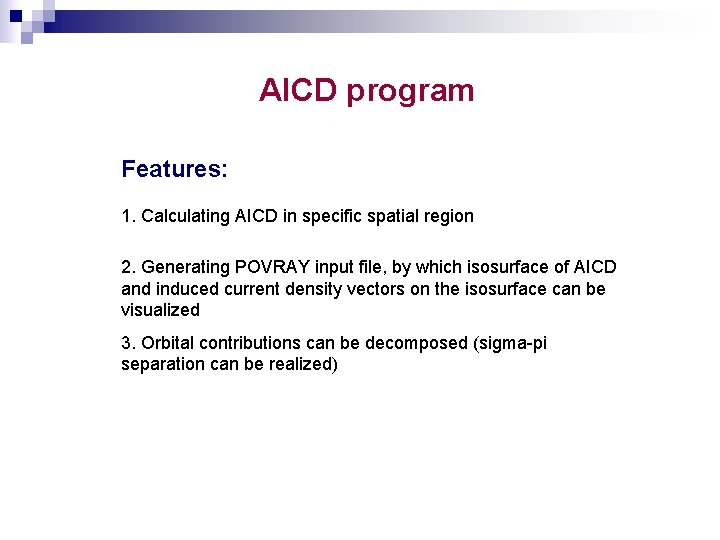
AICD program Features: 1. Calculating AICD in specific spatial region 2. Generating POVRAY input file, by which isosurface of AICD and induced current density vectors on the isosurface can be visualized 3. Orbital contributions can be decomposed (sigma-pi separation can be realized)

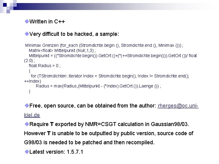
u. Written in C++ u. Very difficult to be hacked, a sample: Minimax Grenzen (for_each (Stromdichte. begin (), Stromdichte. end (), Minimax ())) ; Matrix<float> Mittelpunkt (Null, 1, 3) ; Mittelpunkt = ((*Stromdichte. begin()). Get. Ort ()+(*(++Stromdichte. begin())). Get. Ort ())/ float (2. 0) ; float Radius = 0 ; { for (TStromdichten: : iterator Index = Stromdichte. begin(); Index != Stromdichte. end(); ++Index) Radius = max(Radius, (Mittelpunkt - (*Index). Get. Ort ()). Laenge ()) ; } u. Free, open source, can be obtained from the author: rherges@oc. unikiel. de u. Require T exported by NMR=CSGT calculation in Gaussian 98/03. However T is unable to be outputted by public version, source code of G 98/03 is needed to be patched and then recompiled. u. Latest version: 1. 5. 7. 1

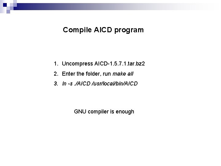
Compile AICD program 1. Uncompress AICD-1. 5. 7. 1. tar. bz 2 2. Enter the folder, run make all 3. ln -s. /AICD /usr/local/bin/AICD GNU compiler is enough

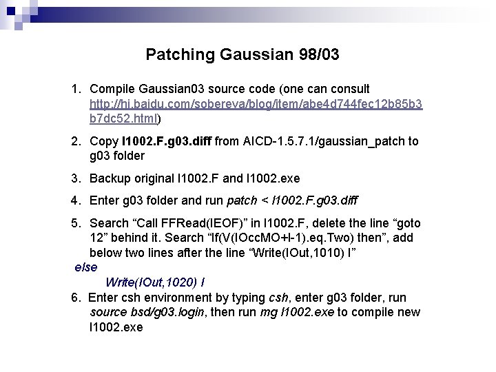
Patching Gaussian 98/03 1. Compile Gaussian 03 source code (one can consult http: //hi. baidu. com/sobereva/blog/item/abe 4 d 744 fec 12 b 85 b 3 b 7 dc 52. html) 2. Copy l 1002. F. g 03. diff from AICD-1. 5. 7. 1/gaussian_patch to g 03 folder 3. Backup original l 1002. F and l 1002. exe 4. Enter g 03 folder and run patch < l 1002. F. g 03. diff 5. Search “Call FFRead(IEOF)” in l 1002. F, delete the line “goto 12” behind it. Search “If(V(IOcc. MO+I-1). eq. Two) then”, add below two lines after the line “Write(IOut, 1010) I” else Write(IOut, 1020) I 6. Enter csh environment by typing csh, enter g 03 folder, run source bsd/g 03. login, then run mg l 1002. exe to compile new l 1002. exe

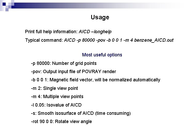
Usage Print full help information: AICD –longhelp Typical command: AICD -p 80000 -pov -b 0 0 1 -m 4 benzene_AICD. out Most useful options -p 80000: Number of grid points -pov: Output input file of POVRAY render -b 0 0 1: Magnetic field vector, will be normalized automatically -m 2: Single view point -m 4: Multiple view points -l 0. 05: Isovalue of AICD -s: Smooth isosurface of AICD (time consuming) -rot 90 0 0: Rotate view angle

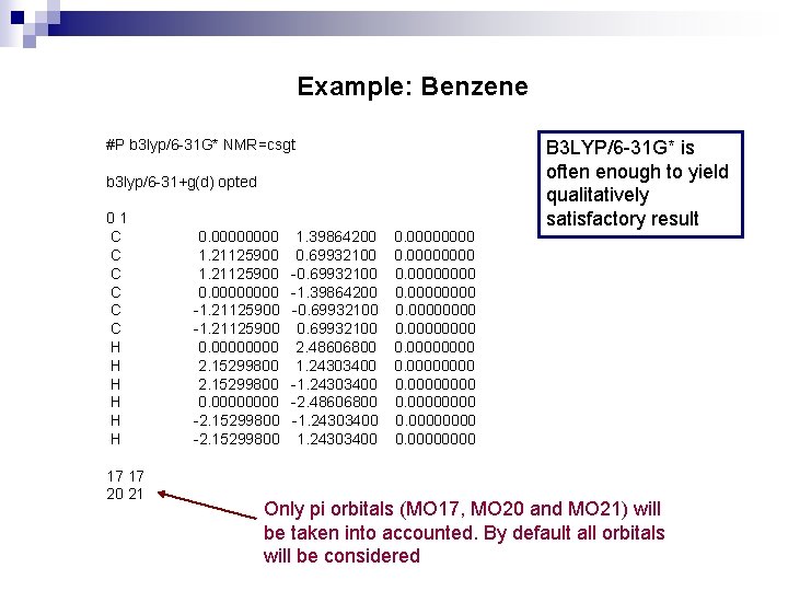
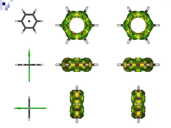
Example: Benzene #P b 3 lyp/6 -31 G* NMR=csgt b 3 lyp/6 -31+g(d) opted 01 C C C H H H 17 17 20 21 0. 0000 1. 21125900 0. 0000 -1. 21125900 0. 0000 2. 15299800 0. 0000 -2. 15299800 1. 39864200 0. 69932100 -1. 39864200 -0. 69932100 2. 48606800 1. 24303400 -2. 48606800 -1. 24303400 0. 00000000 0. 00000000 B 3 LYP/6 -31 G* is often enough to yield qualitatively satisfactory result Only pi orbitals (MO 17, MO 20 and MO 21) will be taken into accounted. By default all orbitals will be considered

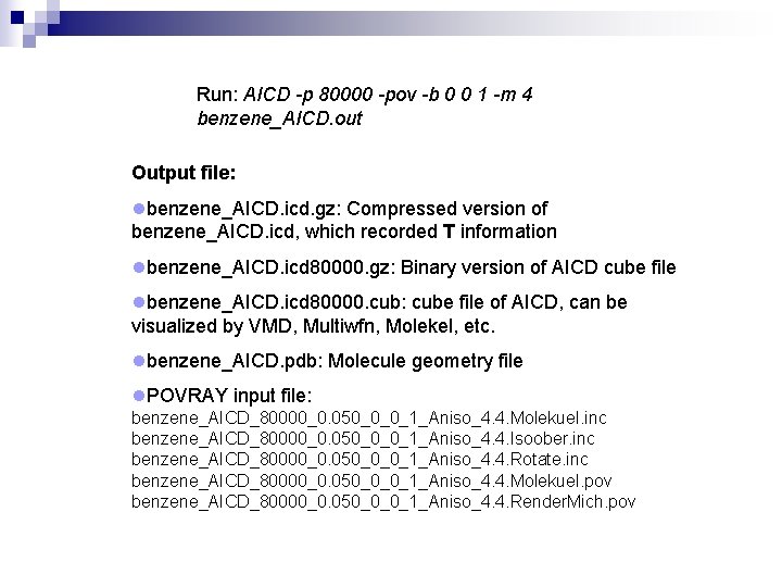
Run: AICD -p 80000 -pov -b 0 0 1 -m 4 benzene_AICD. out Output file: lbenzene_AICD. icd. gz: Compressed version of benzene_AICD. icd, which recorded T information lbenzene_AICD. icd 80000. gz: Binary version of AICD cube file lbenzene_AICD. icd 80000. cub: cube file of AICD, can be visualized by VMD, Multiwfn, Molekel, etc. lbenzene_AICD. pdb: Molecule geometry file l. POVRAY input file: benzene_AICD_80000_0. 050_0_0_1_Aniso_4. 4. Molekuel. inc benzene_AICD_80000_0. 050_0_0_1_Aniso_4. 4. Isoober. inc benzene_AICD_80000_0. 050_0_0_1_Aniso_4. 4. Rotate. inc benzene_AICD_80000_0. 050_0_0_1_Aniso_4. 4. Molekuel. pov benzene_AICD_80000_0. 050_0_0_1_Aniso_4. 4. Render. Mich. pov

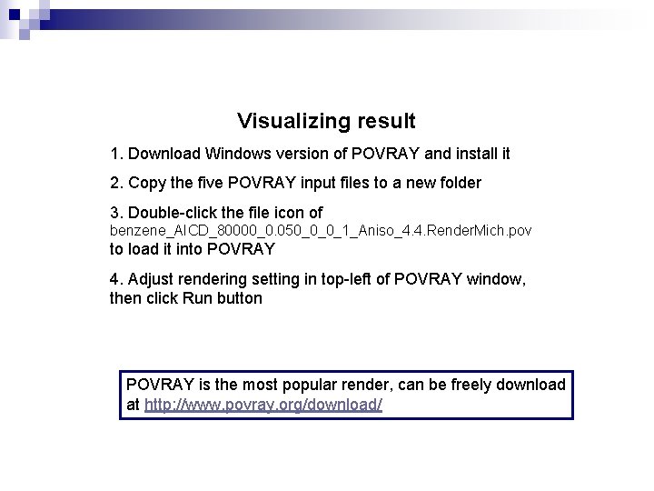
Visualizing result 1. Download Windows version of POVRAY and install it 2. Copy the five POVRAY input files to a new folder 3. Double-click the file icon of benzene_AICD_80000_0. 050_0_0_1_Aniso_4. 4. Render. Mich. pov to load it into POVRAY 4. Adjust rendering setting in top-left of POVRAY window, then click Run button POVRAY is the most popular render, can be freely download at http: //www. povray. org/download/

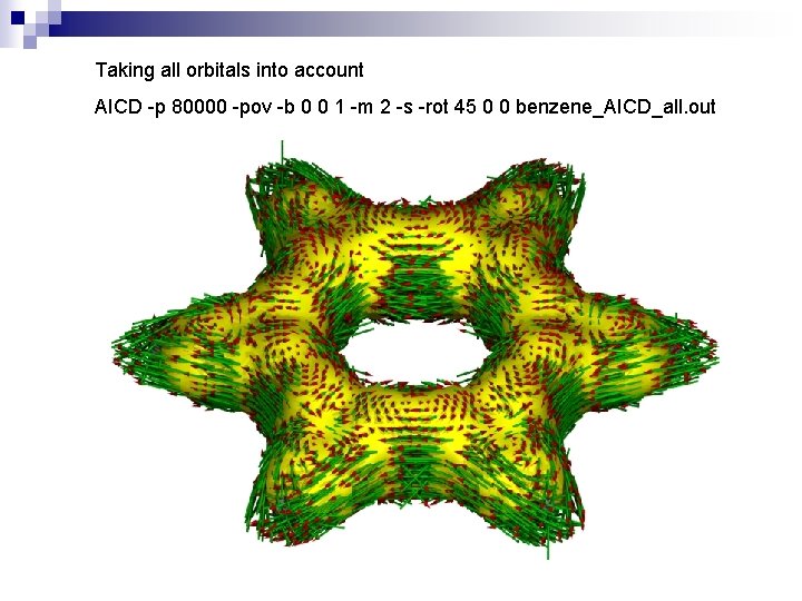
Taking all orbitals into account AICD -p 80000 -pov -b 0 0 1 -m 2 -s -rot 45 0 0 benzene_AICD_all. out

For more details about AICD, see Chem. Rev. , 105, 3758 http: //hi. baidu. com/sobereva/blog/item/88 b 6 fa 544 c 64 e 43 e 3 a 293581. html

GIMIC program Functions: 1. Outputting induced current density, its modulus, divergence in specific 2 D plane or 3 D spatial region 2. Outputting electron density in specific 2 D plane or 3 D spatial region 3. Integration of the current flow through defined cut-planes in molecules

l. Written in Fortran 90, easy to be hacked l. Free, open source, can be downloaded at https: //gitorious. org/gimic l. Principally can be interfaced to any quantum chemistry programs that with GIAO implmented. Currently only interfaced to CFOUR/ACESII and Turbomole l. Unable to decompose orbital contribution like AICD

Digression: A brief introduction of CFOUR Main page: http: //www. cfour. de Manual: http: //slater. chemie. uni-mainz. de/cfour/index. php? n=Main. Manual u. CFOUR=Coupled-Cluster techniques for Computational Chemistry u. Renamed from ACESII-MAB, which is a variant of ACESII u. Free, open source, but fax or regular mail is mandatory to apply a license u. High efficient coupled-cluster calculation, analytic derivatives are available for many sophisticated theoretical methods u. Interface to GIMIC, MRCC, DIRAC, NEWTON-X u. Lacking of a well written manual

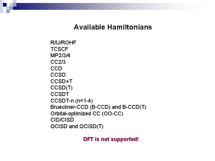
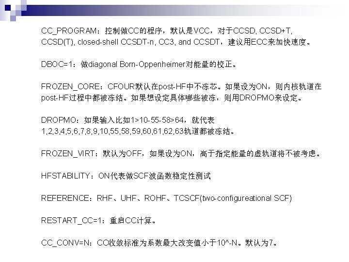
Available Hamiltonians R/U/ROHF TCSCF MP 2/3/4 CC 2/3 CCD CCSD+T CCSD(T) CCSDT-n (n=1 -4) Brueckner-CCD (B-CCD) and B-CCD(T) Orbital-optimized CC (OO-CC) CID/CISD QCISD and QCISD(T) DFT is not supported!

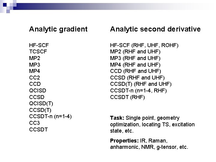
Analytic gradient Analytic second derivative HF-SCF TCSCF MP 2 MP 3 MP 4 CC 2 CCD QCISD CCSD QCISD(T) CCSDT-n (n=1 -4) CC 3 CCSDT HF-SCF (RHF, UHF, ROHF) MP 2 (RHF and UHF) MP 3 (RHF and UHF) MP 4 (RHF and UHF) CCD (RHF and UHF) CCSD(T) (RHF and UHF) CCSDT-n (n=1 -4, RHF) CCSDT (RHF) Task: Single point, geometry optimization, locating TS, excitation state, etc. Properties: IR, Raman, anharmonic, NMR, g-tensor, etc.

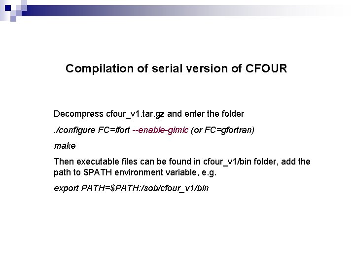
Compilation of serial version of CFOUR Decompress cfour_v 1. tar. gz and enter the folder. /configure FC=ifort --enable-gimic (or FC=gfortran) make Then executable files can be found in cfour_v 1/bin folder, add the path to $PATH environment variable, e. g. export PATH=$PATH: /sob/cfour_v 1/bin

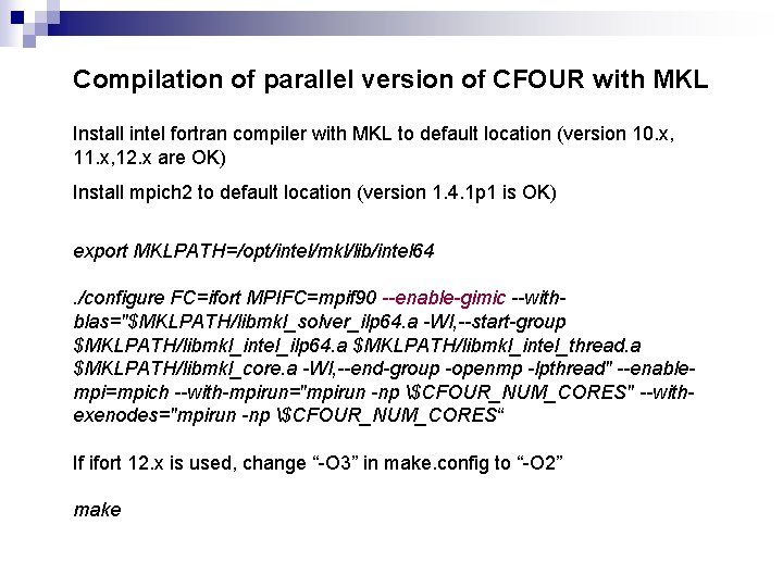
Compilation of parallel version of CFOUR with MKL Install intel fortran compiler with MKL to default location (version 10. x, 11. x, 12. x are OK) Install mpich 2 to default location (version 1. 4. 1 p 1 is OK) export MKLPATH=/opt/intel/mkl/lib/intel 64. /configure FC=ifort MPIFC=mpif 90 --enable-gimic --withblas="$MKLPATH/libmkl_solver_ilp 64. a -Wl, --start-group $MKLPATH/libmkl_intel_ilp 64. a $MKLPATH/libmkl_intel_thread. a $MKLPATH/libmkl_core. a -Wl, --end-group -openmp -lpthread" --enablempi=mpich --with-mpirun="mpirun -np $CFOUR_NUM_CORES" --withexenodes="mpirun -np $CFOUR_NUM_CORES“ If ifort 12. x is used, change “-O 3” in make. config to “-O 2” make

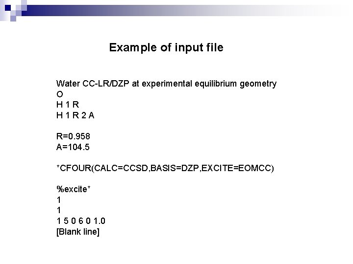
Example of input file Water CC-LR/DZP at experimental equilibrium geometry O H 1 R 2 A R=0. 958 A=104. 5 *CFOUR(CALC=CCSD, BASIS=DZP, EXCITE=EOMCC) %excite* 1 1 1 5 0 6 0 1. 0 [Blank line]

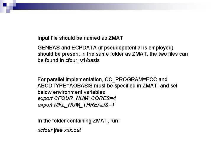
Input file should be named as ZMAT GENBAS and ECPDATA (if pseudopotential is employed) should be present in the same folder as ZMAT, the two files can be found in cfour_v 1/basis For parallel implementation, CC_PROGRAM=ECC and ABCDTYPE=AOBASIS must be specified in ZMAT, and set below environment variables export CFOUR_NUM_CORES=4 export MKL_NUM_THREADS=1 In the folder containing ZMAT, run: xcfour |tee xxx. out

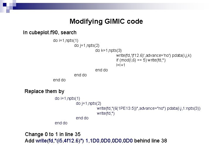
Modifying GIMIC code In cubeplot. f 90, search do i=1, npts(1) do j=1, npts(2) do k=1, npts(3) write(fd, '(f 12. 6)', advance='no') pdata(i, j, k) if (mod(l, 6) == 5) write(fd, *) l=l+1 end do Replace them by do i=1, npts(1) do j=1, npts(2) write(fd, "(6(1 PE 13. 5))", advance="no") pdata(i, j, 1: npts(3)) write(fd, *) end do Change 0 to 1 in line 35 Add write(fd, "(i 5, 4 f 12. 6)") 1, 1 D 0, 0 D 0 behind line 38

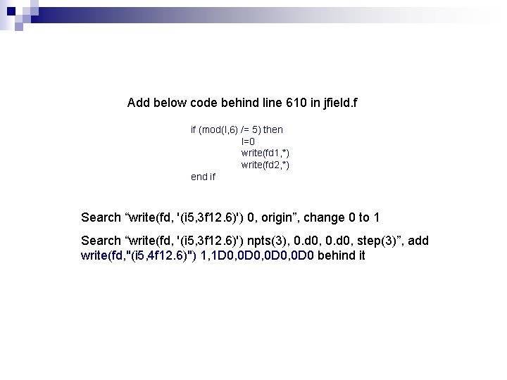
Add below code behind line 610 in jfield. f if (mod(l, 6) /= 5) then l=0 write(fd 1, *) write(fd 2, *) end if Search “write(fd, '(i 5, 3 f 12. 6)') 0, origin”, change 0 to 1 Search “write(fd, '(i 5, 3 f 12. 6)') npts(3), 0. d 0, step(3)”, add write(fd, "(i 5, 4 f 12. 6)") 1, 1 D 0, 0 D 0 behind it

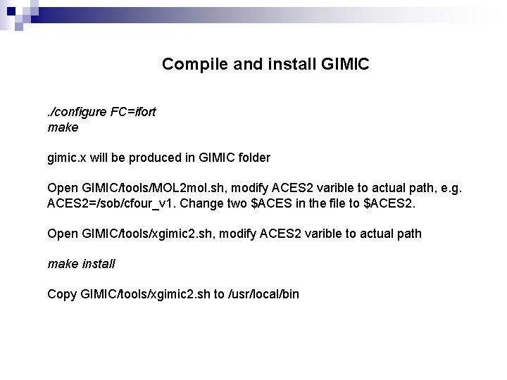
Compile and install GIMIC. /configure FC=ifort make gimic. x will be produced in GIMIC folder Open GIMIC/tools/MOL 2 mol. sh, modify ACES 2 varible to actual path, e. g. ACES 2=/sob/cfour_v 1. Change two $ACES in the file to $ACES 2. Open GIMIC/tools/xgimic 2. sh, modify ACES 2 varible to actual path make install Copy GIMIC/tools/xgimic 2. sh to /usr/local/bin

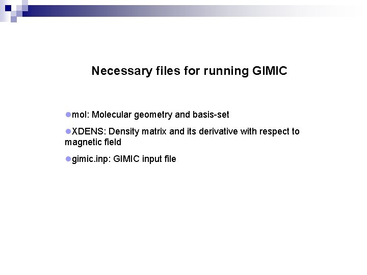
Necessary files for running GIMIC lmol: Molecular geometry and basis-set l. XDENS: Density matrix and its derivative with respect to magnetic field lgimic. inp: GIMIC input file

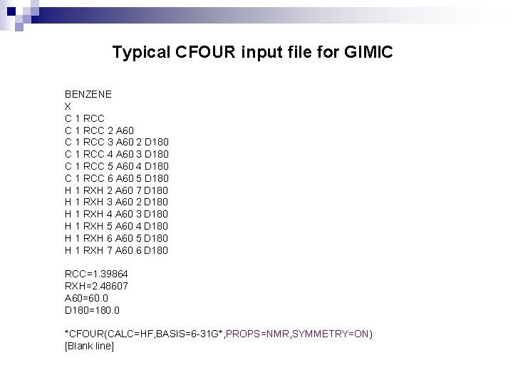
Typical CFOUR input file for GIMIC BENZENE X C 1 RCC 2 A 60 C 1 RCC 3 A 60 2 D 180 C 1 RCC 4 A 60 3 D 180 C 1 RCC 5 A 60 4 D 180 C 1 RCC 6 A 60 5 D 180 H 1 RXH 2 A 60 7 D 180 H 1 RXH 3 A 60 2 D 180 H 1 RXH 4 A 60 3 D 180 H 1 RXH 5 A 60 4 D 180 H 1 RXH 6 A 60 5 D 180 H 1 RXH 7 A 60 6 D 180 RCC=1. 39864 RXH=2. 48607 A 60=60. 0 D 180=180. 0 *CFOUR(CALC=HF, BASIS=6 -31 G*, PROPS=NMR, SYMMETRY=ON) [Blank line]

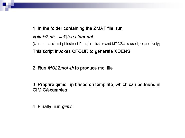
1. In the folder containing the ZMAT file, run xgimic 2. sh --scf |tee cfour. out (Use --cc and –mbpt instead if couple-cluster and MP 2/3/4 is used, respectively) This script invokes CFOUR to generate XDENS 2. Run MOL 2 mol. sh to produce mol file 3. Prepare gimic. inp based on template, which can be found in GIMIC/examples 4. Finally, run gimic

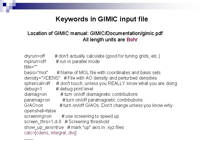
Keywords in GIMIC input file Location of GIMIC manual: GIMIC/Documentation/gimic. pdf All length units are Bohr dryrun=off # don't actually calculate (good for tuning grids, etc. ) mpirun=off # run in parallel mode title="" basis="mol" # Name of MOL file with coordinates and basis sets density="XDENS" # File with AO density and perturbed densities spherical=off # don't touch, unless you REALLY know what you are doing debug=1 # debug print level diamag=on # turn on/off diamagnetic contributions paramag=on # turn on/off paramagnetic contributions GIAO=on # turn on/off GIAOs. Don't change unless you know why. openshell=false screening=on # use screening to speed up screen_thrs=1. d-8 # Screening threshold show_up_axis=true # mark "up" axis in. xyz files calc=[cdens, integral, divj] ……

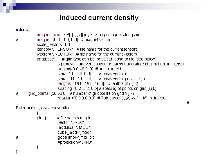
Induced current density cdens { # # magnet_axis=-z #[-] i, j, k || x, y, z -> align magnet along axis magnet=[0. 0, -1. 0, 0. 0] # magnet vector scale_vectors=1. 0 jtensor="JTENSOR" # file name for the current tensors jvector="JVECTOR" # file name for the current vectors grid(base) { # grid type can be: base/std, bond or file (see below) type=even # even spaced or gauss quadrature distribution on interval origin=[-8. 0, 0] # origin of grid ivec=[1. 0, 0. 0] # basis vector i jvec=[ 0. 0, 1. 0, 0. 0] # basis vector j ( k = i x j ) lengths=[16. 0, 16. 0] # lenthts of (i, j, k) spacing=[0. 2, 0. 5] # spacing of points on grid (i, j, k) grid_points=[50, 0] # number of gridpoints on grid (i, j, k) rotation=[0. 0, 0. 0] # Rotation of (i, j, k) -> (i', j', k') in degrees # Euler angles, x-y-z convention } plot { # file names for plots vector="JVEC" modulus="JMOD" cube_mod="jmod" # gopenmol="jmod. plt" #projection="JPRJ" } }

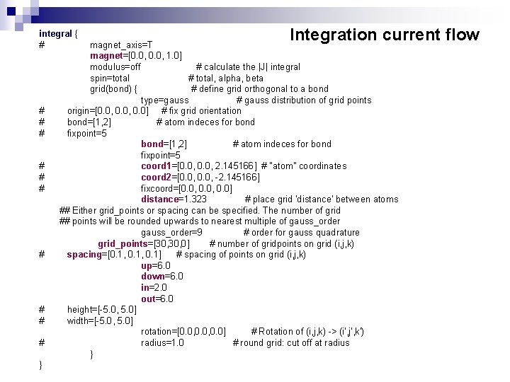
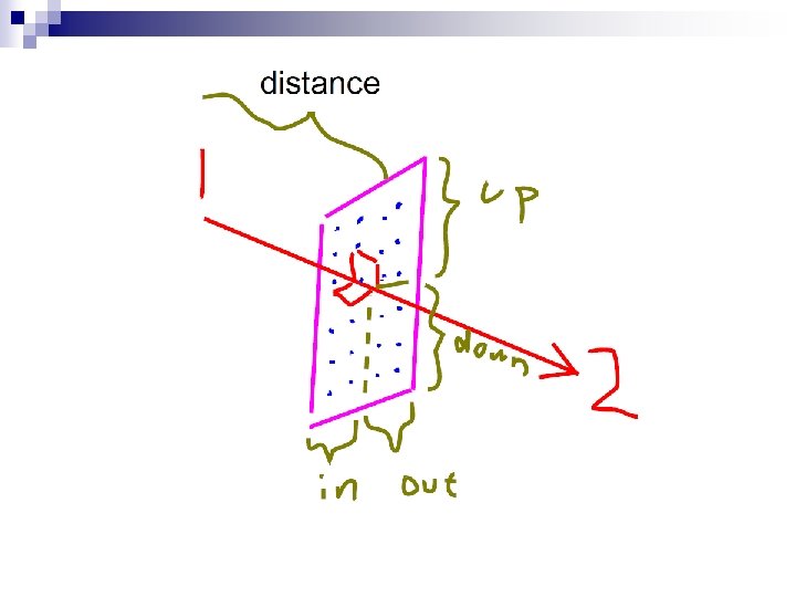
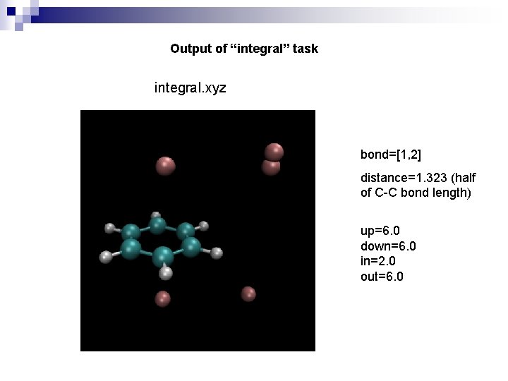
integral { # # # } Integration current flow magnet_axis=T magnet=[0. 0, 1. 0] modulus=off # calculate the |J| integral spin=total # total, alpha, beta grid(bond) { # define grid orthogonal to a bond type=gauss # gauss distribution of grid points origin=[0. 0, 0. 0] # fix grid orientation bond=[1, 2] # atom indeces for bond fixpoint=5 coord 1=[0. 0, 2. 145166] # "atom" coordinates coord 2=[0. 0, -2. 145166] fixcoord=[0. 0, 0. 0] distance=1. 323 # place grid 'distance' between atoms ## Either grid_points or spacing can be specified. The number of grid ## points will be rounded upwards to nearest multiple of gauss_order=9 # order for gauss quadrature grid_points=[30, 0] # number of gridpoints on grid (i, j, k) spacing=[0. 1, 0. 1] # spacing of points on grid (i, j, k) up=6. 0 down=6. 0 in=2. 0 out=6. 0 height=[-5. 0, 5. 0] width=[-5. 0, 5. 0] rotation=[0. 0, 0. 0] # Rotation of (i, j, k) -> (i', j', k') radius=1. 0 # round grid: cut off at radius }

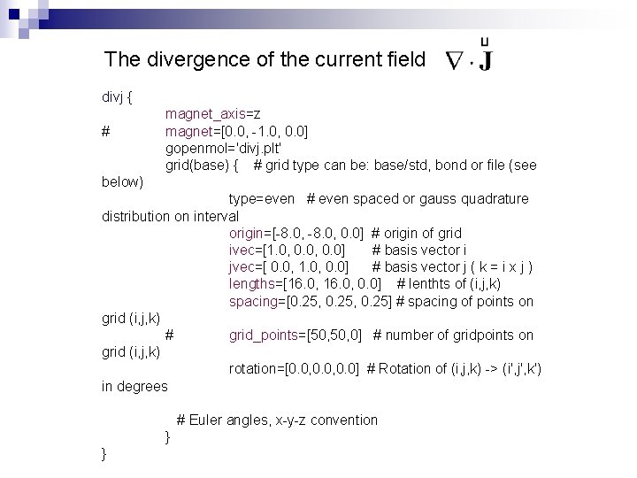
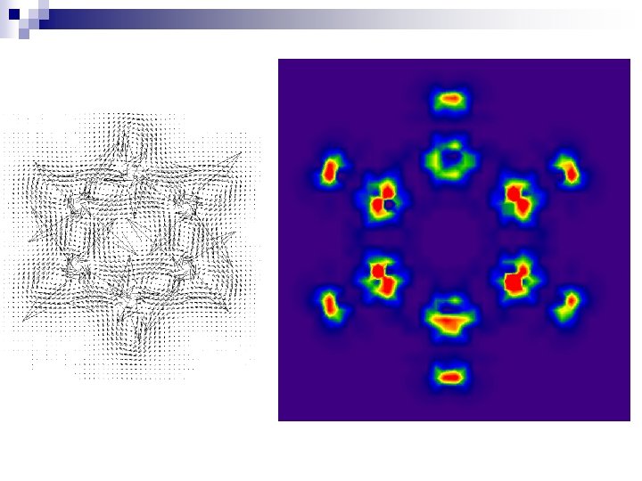
The divergence of the current field divj { # magnet_axis=z magnet=[0. 0, -1. 0, 0. 0] gopenmol='divj. plt' grid(base) { # grid type can be: base/std, bond or file (see below) type=even # even spaced or gauss quadrature distribution on interval origin=[-8. 0, 0. 0] # origin of grid ivec=[1. 0, 0. 0] # basis vector i jvec=[ 0. 0, 1. 0, 0. 0] # basis vector j ( k = i x j ) lengths=[16. 0, 0. 0] # lenthts of (i, j, k) spacing=[0. 25, 0. 25] # spacing of points on grid (i, j, k) # grid_points=[50, 0] # number of gridpoints on grid (i, j, k) rotation=[0. 0, 0. 0] # Rotation of (i, j, k) -> (i', j', k') in degrees # Euler angles, x-y-z convention } }

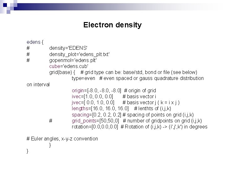
Electron density edens { # # # density='EDENS' density_plot='edens_plt. txt' gopenmol='edens. plt' cube='edens. cub' grid(base) { # grid type can be: base/std, bond or file (see below) type=even # even spaced or gauss quadrature distribution on interval origin=[-8. 0, -8. 0] # origin of grid ivec=[1. 0, 0. 0] # basis vector i jvec=[ 0. 0, 1. 0, 0. 0] # basis vector j ( k = i x j ) lengths=[16. 0, 16. 0] # lenthts of (i, j, k) spacing=[0. 2, 0. 2] # spacing of points on grid (i, j, k) # grid_points=[50, 0] # number of gridpoints on grid (i, j, k) rotation=[0. 0, 0. 0] # Rotation of (i, j, k) -> (i', j', k') in degrees # Euler angles, x-y-z convention } }

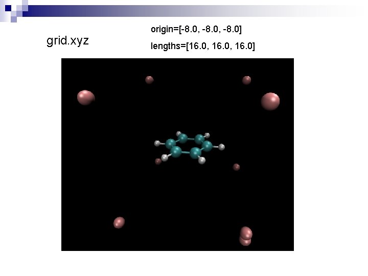
grid. xyz origin=[-8. 0, -8. 0] lengths=[16. 0, 16. 0]

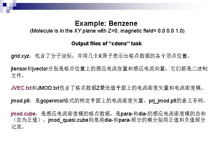
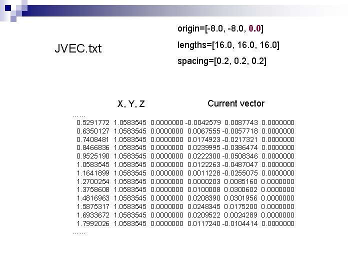
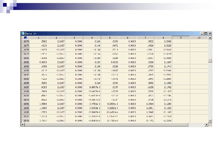
origin=[-8. 0, 0. 0] lengths=[16. 0, 16. 0] JVEC. txt spacing=[0. 2, 0. 2] X, Y, Z …… 0. 5291772 0. 6350127 0. 7408481 0. 8466836 0. 9525190 1. 0583545 1. 1641899 1. 2700254 1. 3758608 1. 4816963 1. 5875317 1. 6933672 1. 7992026 …… 1. 0583545 1. 0583545 Current vector 0. 0000000 -0. 0042579 0. 0087743 0. 0000000 0. 0067555 -0. 0057718 0. 0000000 0. 0174923 -0. 0217321 0. 0000000 0. 0239995 -0. 0386474 0. 0000000 0. 0222300 -0. 0508346 0. 0000000 0. 0122263 -0. 0487047 0. 0000000 0. 0011228 -0. 0255075 0. 0000000 0. 0000203 0. 0085160 0. 0000000 0. 0100008 0. 0300602 0. 0000000 0. 0208390 0. 0301956 0. 0000000 0. 0248345 0. 0175200 0. 0000000 0. 0209522 0. 0024289 0. 0000000 0. 0117240 -0. 0104414 0. 0000000 0. 0000000

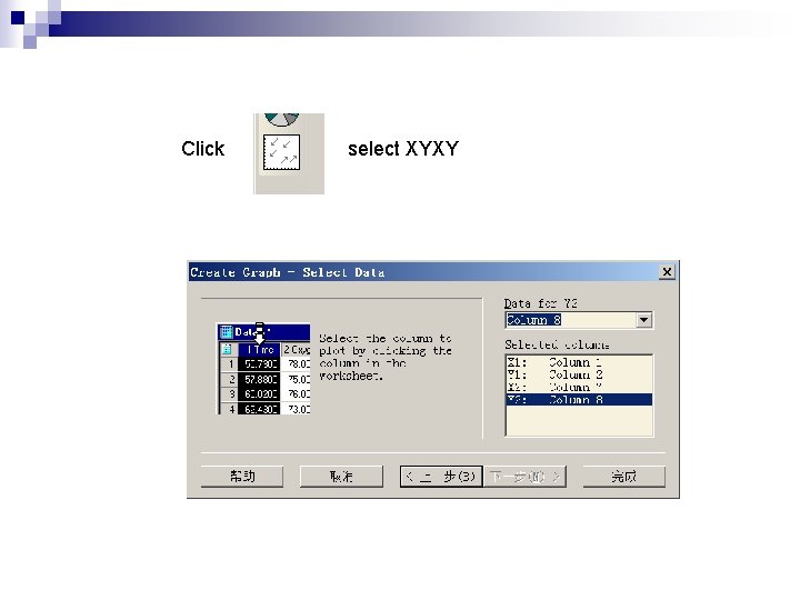
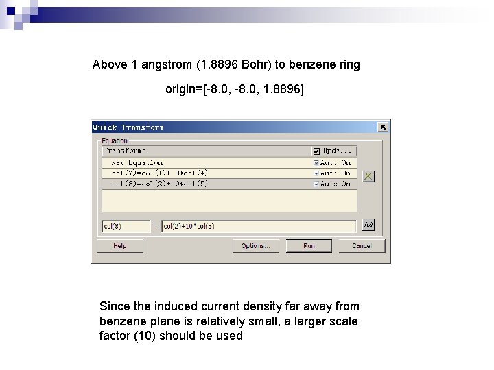
Plotting JVEC. txt by Sigmaplot 11 1. Create a new note book 2. File-Import-File, select JVEC. txt, click import button 3. Transform-Quick transform, input formula and click Run button

Click select XYXY

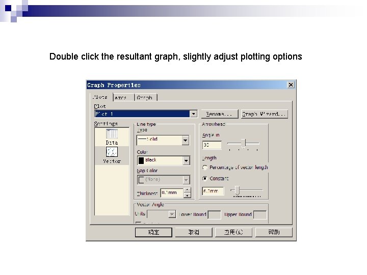
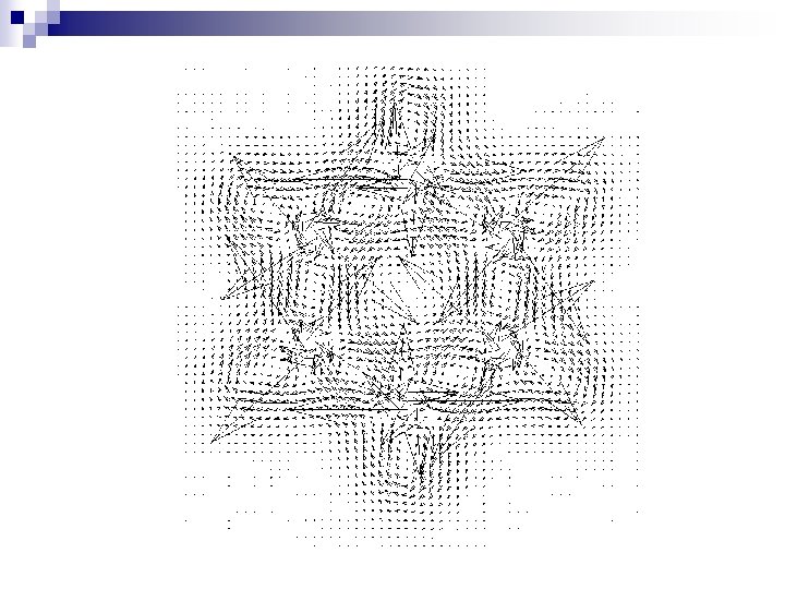
Double click the resultant graph, slightly adjust plotting options

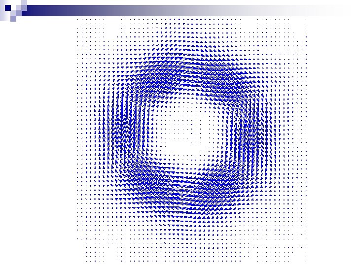
Above 1 angstrom (1. 8896 Bohr) to benzene ring origin=[-8. 0, 1. 8896] Since the induced current density far away from benzene plane is relatively small, a larger scale factor (10) should be used

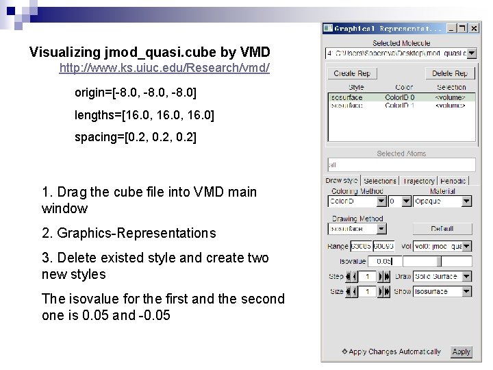
Visualizing jmod_quasi. cube by VMD http: //www. ks. uiuc. edu/Research/vmd/ origin=[-8. 0, -8. 0] lengths=[16. 0, 16. 0] spacing=[0. 2, 0. 2] 1. Drag the cube file into VMD main window 2. Graphics-Representations 3. Delete existed style and create two new styles The isovalue for the first and the second one is 0. 05 and -0. 05

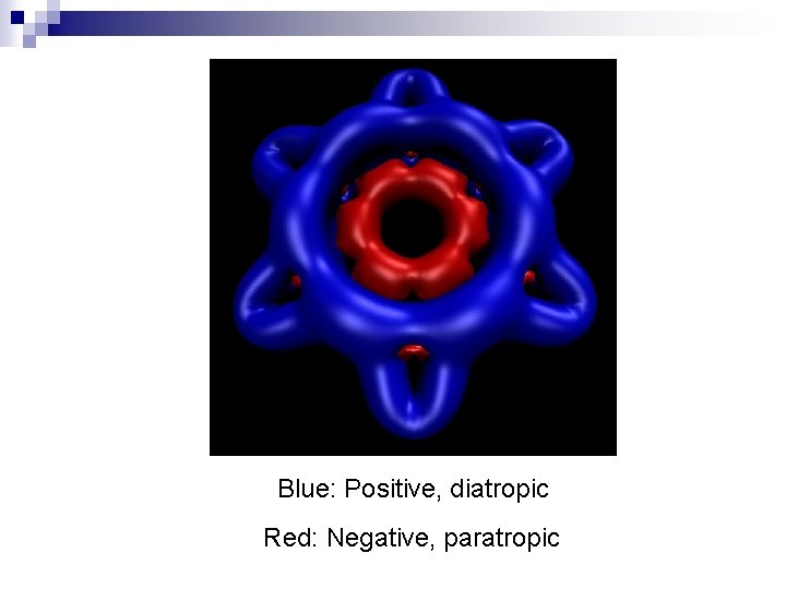
Blue: Positive, diatropic Red: Negative, paratropic

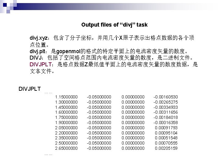
Output files of “divj” task divj. xyz：包含了分子坐标，并用几个X原子表示出格点数据的各个顶 点位置。 divj. plt：是gopenmol的格式的特定平面上的电流密度矢量的散度。 DIVJ：包括了空间格点范围内电流密度矢量的散度，是二进制文件。 DIVJPLT：是格点数据Z最低值平面上的电流密度矢量的散度数据，是 文本文件。 DIVJPLT …… 1. 15000000 1. 30000000 1. 45000000 1. 60000000 1. 75000000 1. 90000000 2. 05000000 2. 20000000 2. 35000000 2. 50000000 2. 65000000 …… -0. 05000000 -0. 05000000 0. 00000000 0. 0000 -0. 00160530 -0. 00265275 -0. 00334933 -0. 00311656 -0. 00184018 -0. 00016358 0. 00091793 0. 00095104 0. 00051548 0. 00070555 0. 00205159

Plotting DIVJPLT by Sigmaplot 11 1. Rename it to DIVJPLT. txt 2. Import DIVJPLT. txt into Sigmaplot 11 3. Make quick transformation: col(5)=abs(col(4)) 4. 5. Select XYZ Triplet

Output of “integral” task integral. xyz bond=[1, 2] distance=1. 323 (half of C-C bond length) up=6. 0 down=6. 0 in=2. 0 out=6. 0

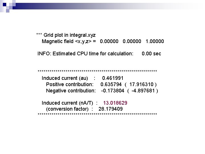
*** Grid plot in integral. xyz Magnetic field <x, y, z> = 0. 00000 1. 00000 INFO: Estimated CPU time for calculation: 0. 00 sec ****************************** Induced current (au) : 0. 461991 Positive contribution: 0. 635794 ( 17. 916310 ) Negative contribution: -0. 173804 ( -4. 897681 ) Induced current (n. A/T) : 13. 018629 (conversion factor) : 28. 179409 ******************************

Notes for GIMIC calculation ØAccurate current densities can generally be obtained at the DFT level, using standard double-zeta basis sets augmented with polarization functions ØSpin currents are much more sensitive to the employed computational level and the size of the basis set. ØElectron correlation should be considered in openshell calculations, CCSD is robost, DFT may be OK, and large basis sets (triple-zeta) have to be employed