UNITI Introduction to Matlab MATLAB stands for Matrix

UNIT-I

Introduction to Matlab

• MATLAB stands for Matrix Laboratory. • MATLAB had many functions and toolboxes to help in various applications • It allows you to solve many technical computing problems, especially those with matrix and vector formulas, in a fraction of the time it would take to write a program in a scalar non-interactive language such as C or Fortran.

MATLAB is basically a high level language which has many specialized toolboxes for making things easier for us. Matlab High Level Languages such as C, Pascal etc. Assembly

The MATLAB System MATLAB system consists of these main parts: • Desktop Tools and Development Environment – Includes the MATLAB desktop and Command Window, an editor and debugger, a code analyzer, browsers for viewing help, the workspace, files, and other tools • Mathematical Function Library – vast collection of computational algorithms ranging from elementary functions, like sine, cosine, and complex arithmetic, to more sophisticated functions like matrix inverse, matrix eigenvalues, Bessel functions, and fast Fourier transforms.

• The Language – The MATLAB language is a high-level matrix/array language with control flow statements, functions, data structures, input/output, and object-oriented programming features. • Graphics – MATLAB has extensive facilities for displaying vectors and matrices as graphs, as well as editing and printing these graphs. It also includes functions that allow you to customize the appearance of graphics as well as build complete graphical user interfaces on your MATLAB applications. • External Interfaces – The external interfaces library allows you to write C and Fortran programs that interact with MATLAB.

Matlab Screen • Command Window – type commands • Current Directory – View folders and m-files • Workspace – View program variables – Double click on a variable to see it in the Array Editor • Command History – view past commands – save a whole session using diary
 entities in MATLAB are matrices •")
Working with Matrices and Arrays • All (almost) entities in MATLAB are matrices • Easy to define • Separate the elements of a row with blanks(‘ ‘)or commas (‘ , ’). • Use a semicolon ( ; ) to indicate the end of each row. • Surround the entire list of elements with square brackets, [ ].

A = [16 3 2 13; 5 10 11 8; 9 6 7 12; 4 15 14 1] • MATLAB displays the matrix you just entered: A = 16 3 2 13 5 10 11 8 9 6 7 12 4 15 14 1 • Once you have entered the matrix, it is automatically remembered in the MATLAB workspace. You can simply refer to it as A. • Keep in mind, variable names are case-sensitive

The Colon Operator For example: 1 : 10 is a row vector containing the integers from 1 to 10: 1 2 3 4 5 6 7 8 9 10 • To obtain non-unit spacing, specify an increment. For example: 100 : -7 : 50 will give you 100 93 86 79 72 65 58 51
![Creating Vectors and Matrices • Define >> A = [16 3; 5 10] A](http://slidetodoc.com/presentation_image_h/2f2e983e7c3f717107daad2d5a702c07/image-12.jpg "Creating Vectors and Matrices • Define >> A = [16 3; 5 10] A")
Creating Vectors and Matrices • Define >> A = [16 3; 5 10] A = 16 3 5 10 >> B = [3 4 5; 6 7 8] • Transpose Vector : >> a=[1 2 3]; >> a' 1 2 3 B = 3 6 4 7 5 8 Matrix: >> A=[1 2; 3 4]; >> A' 1 3 2 4
: matrix with all zeros • ones(m, n):")
Generating Vectors from functions • zeros(m, n): matrix with all zeros • ones(m, n): matrix with all ones. • eye(m, n): the identity matrix • rand(m, n): uniformly distributed random • randn(m, n): normally distributed random

Matrix operations • ^: exponentiation • *: multiplication • /: division • : left division. The operation AB is effectively the same as INV(A)*B, although left division is calculated differently and is much quicker. • +: addition • -: subtraction
. ^")
Array Operations • Evaluated element by element. ' : array transpose (non-conjugated transpose). ^ : array power. * : array multiplication. / : array division • Very different from Matrix operations >> A=[1 2; 3 4]; >> B=[5 6; 7 8]; >> A*B 19 22 43 50 But: >> A. *B 5 21 12 32
: mean value of a vector • max(A), min (A):")
Some Built-in functions • mean(A): mean value of a vector • max(A), min (A): maximum and minimum. • sum(A): summation. • sort(A): sorted vector • median(A): median value • std(A): standard deviation. • det(A) : determinant of a square matrix • dot(a, b): dot product of two vectors • Cross(a, b): cross product of two vectors • Inv(A): Inverse of a matrix A

Indexing Matrices Given the matrix: n A = m Then: 0. 9501 0. 2311 A(1, 2) = 0. 6068 A(3) = 0. 6068 A(: , 1) = [0. 9501 1: m 0. 2311 ] A(1, 2: 3)=[0. 6068 0. 4231] 0. 6068 0. 4860 0. 4231 0. 2774

Graphics • MATLAB provides a variety of techniques to display data graphically. • Interactive tools enable you to manipulate graphs to achieve results that reveal the most information about your data. • You can also edit and print graphs for presentations, or export graphs to standard graphics formats for presentation in Web browsers or other media.

Basic Plotting Functions • The plot function has different forms, depending on the input arguments. • If y is a vector, plot(y) produces a piecewise graph of the elements of (y) versus the index of the elements of (y). • If you specify two vectors as arguments, plot(x, y) produces a graph of y versus x. • You can also label the axes and add a title, using the ‘xlabel’, ‘ylabel’, and ‘title’ functions. Example: x label ('x = 0: 2pi') y label ('Sine of x') title('Plot of the Sine Function', 'Font. Size', 12)


• Plotting Multiple Data Sets in One Graph – Multiple x-y pair arguments create multiple graphs with a single call to plot. For example: x = 0: pi/100: 2*pi; y = sin(x); y 2 = sin(x-. 25); y 3 = sin(x-. 5); plot(x, y, x, y 2, x, y 3)

• Specifying Line Styles and Colors It is possible to specify color, line styles, and markers (such as plus signs or circles) when you plot your data using the plot command: plot(x, y, 'color_style_marker') For example: plot(x, y, 'r: +') plots a red-dotted line and places plus sign markers at each data point.
 between 0≤x≤ 4π • Create an x-array of")
Basic Task: Plot the function sin(x) between 0≤x≤ 4π • Create an x-array of 100 samples between 0 and 4π. >>x=linspace(0, 4*pi, 100); • Calculate sin(. ) of the x-array >>y=sin(x); • Plot the y-array >>plot(y)
 between 0≤x≤ 4π • Create an x-array of 100")
Plot the function e-x/3 sin(x) between 0≤x≤ 4π • Create an x-array of 100 samples between 0 and 4π. >>x=linspace (0, 4*pi, 100); • Calculate sin(. ) of the x-array >>y=sin(x); • Calculate e-x/3 of the x-array >>y 1=exp(-x/3); • Multiply the arrays y and y 1 >>y 2=y*y 1;
 between 0≤x≤ 4π • Multiply the arrays y and")
Plot the function e-x/3 sin(x) between 0≤x≤ 4π • Multiply the arrays y and y 1 correctly >>y 2=y. *y 1; • Plot the y 2 -array >>plot(y 2)
 Example: >>x=linspace(0, 4*pi, 100); >>y=sin(x); >>plot(y) >>plot(x, y) •")
Display Facilities • plot(. ) Example: >>x=linspace(0, 4*pi, 100); >>y=sin(x); >>plot(y) >>plot(x, y) • stem(. ) Example: >>stem(y) >>stem(x, y)
 >>title(‘This is the sinus function’) • xlabel(. ) >>xlabel(‘x")
Display Facilities • title(. ) >>title(‘This is the sinus function’) • xlabel(. ) >>xlabel(‘x (secs)’) • ylabel(. ) >>ylabel(‘sin(x)’)

subplots • Use subplots to divide a plotting window into several panes. >> >> >> x=0: 0. 1: 10; f=figure; f 1=subplot(1, 2, 1); plot(x, cos(x), 'r'); grid on; title('Cosine') f 2=subplot(1, 2, 2); plot(x, sin(x), 'd'); grid on; title('Sine');
 to save a figure to a file.")
Save plots • Use saveas(h, 'filename. ext') to save a figure to a file. Useful extension types: bmp: Windows bitmap emf: Enhanced metafile >> >> f=figure; x=-5: 0. 1: 5; h=plot(x, cos(2*x+pi/3)); title('Figure 1'); xlabel('x'); saveas(h, 'figure 1. fig') saveas(h, 'figure 1. eps') eps: EPS Level 1 fig: MATLAB figure jpg: JPEG image m: MATLAB M-file tif: TIFF image, compressed

Square Wave close all; clear all; a=input('Enter the amplitude of the square wave A = '); f= input('Enter the frequency of the square wave F = '); dc=input('Enter the duty cycle of the wave DC = '); f=f*2*pi; t=0: . 001: 1; y=a*square(f*t, dc); plot(t, y); axis([0 1 -2 2]);

%output %Enter the amplitude of the square wave A = 2 %Enter the frequency of the square wave F = 10 %Enter the duty cycle of the wave DC = 50
; t=0: n; y=(-1).")
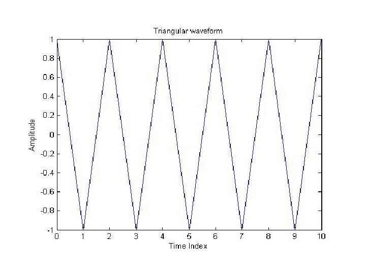
Triangle Wave n=input ('Enter the length of the sequence N= '); t=0: n; y=(-1). ^t; plot(t, y); ylabel ('Amplitude'); xlabel ('Time Index'); TITLE ('Triangular waveform');
- Slides: 33