Unit III Costs of Production and Perfect Competition

Unit III: Costs of Production and Perfect Competition

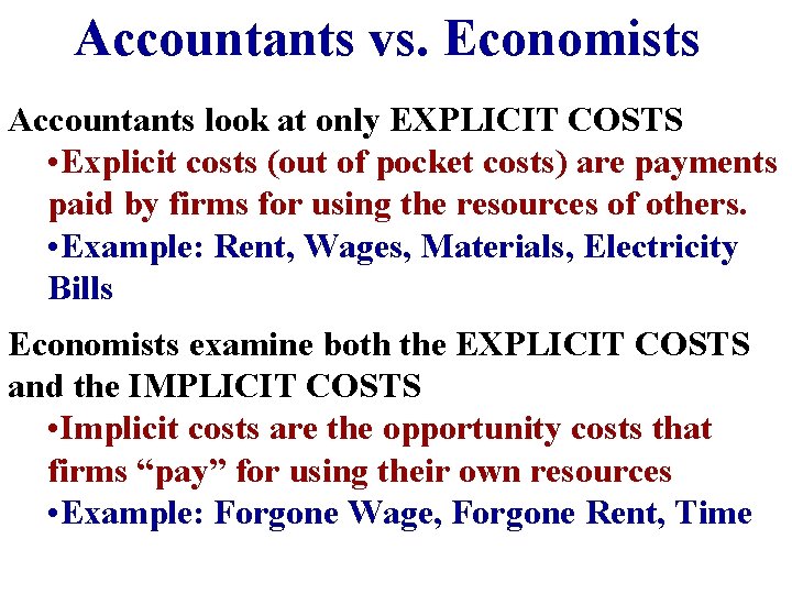
Accountants vs. Economists Accountants look at only EXPLICIT COSTS • Explicit costs (out of pocket costs) are payments paid by firms for using the resources of others. • Example: Rent, Wages, Materials, Electricity Bills Economists examine both the EXPLICIT COSTS and the IMPLICIT COSTS • Implicit costs are the opportunity costs that firms “pay” for using their own resources • Example: Forgone Wage, Forgone Rent, Time

Analyzing Production

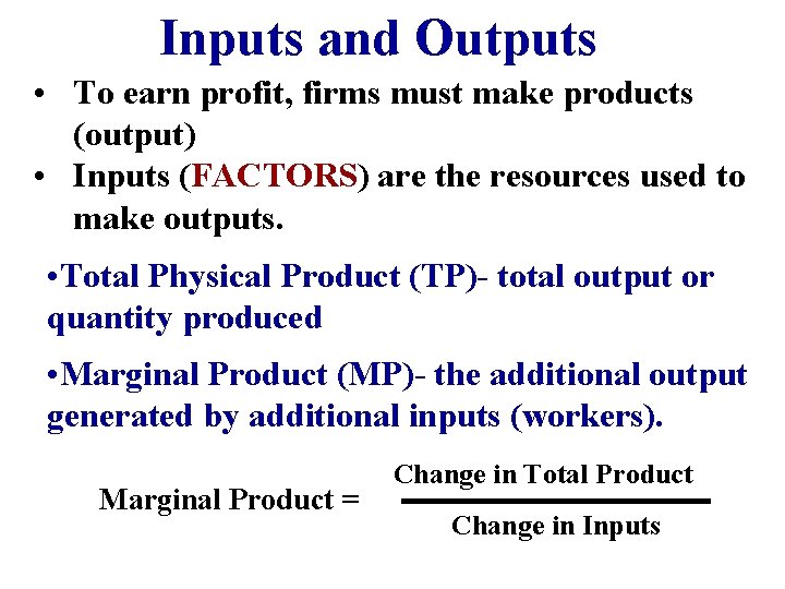
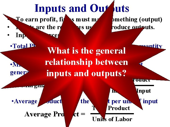
Inputs and Outputs • To earn profit, firms must make products (output) • Inputs (FACTORS) are the resources used to make outputs. • Total Physical Product (TP)- total output or quantity produced • Marginal Product (MP)- the additional output generated by additional inputs (workers). Marginal Product = Change in Total Product Change in Inputs

Inputs and Outputs • To earn profit, firms must make something (output) • Inputs are the resources used to produce outputs. • Input resources are also called FACTORS. • Total Physical Product (TP)- total output or quantity What is the general produced relationship betweenoutput • Marginal Product (MP)- the additional generated byinputs additionaland inputs. outputs? Marginal Product = Change in Total Product Change in Labor Input • Average Product (AP)- the output per unit of input Average Product = Total Product Units of Labor

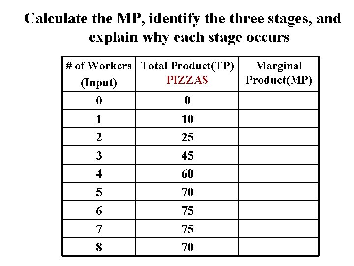
Calculate the MP, identify the three stages, and explain why each stage occurs # of Workers Total Product(TP) Marginal PIZZAS Product(MP) (Input) 0 1 2 3 4 5 6 7 8 0 10 25 45 60 70 75 75 70

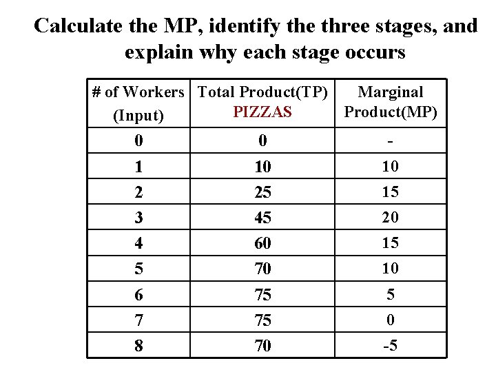
Calculate the MP, identify the three stages, and explain why each stage occurs # of Workers Total Product(TP) Marginal PIZZAS Product(MP) (Input) 0 0 1 2 3 4 5 6 7 8 10 25 45 60 70 75 75 70 10 15 20 15 10 5 0 -5

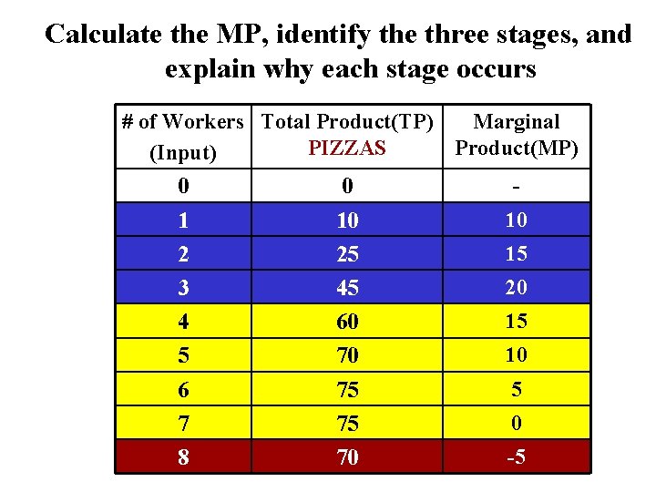
Calculate the MP, identify the three stages, and explain why each stage occurs # of Workers Total Product(TP) Marginal PIZZAS Product(MP) (Input) 0 0 1 2 3 4 5 6 7 8 10 25 45 60 70 75 75 70 10 15 20 15 10 5 0 -5

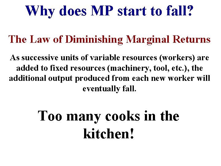
Why does MP start to fall? The Law of Diminishing Marginal Returns As successive units of variable resources (workers) are added to fixed resources (machinery, tool, etc. ), the additional output produced from each new worker will eventually fall. Too many cooks in the kitchen!

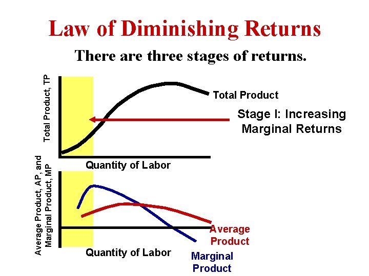
Law of Diminishing Returns Average Product, AP, and Marginal Product, MP Total Product, TP There are three stages of returns. Total Product Stage I: Increasing Marginal Returns Quantity of Labor Average Product Marginal Product

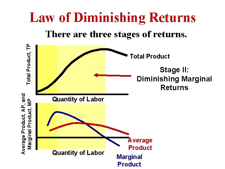
Law of Diminishing Returns Average Product, AP, and Marginal Product, MP Total Product, TP There are three stages of returns. Total Product Stage II: Diminishing Marginal Returns Quantity of Labor Average Product Marginal Product

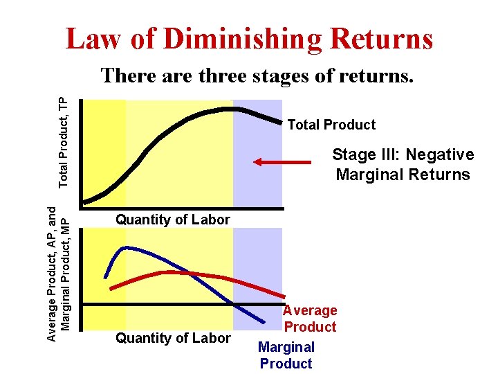
Law of Diminishing Returns Average Product, AP, and Marginal Product, MP Total Product, TP There are three stages of returns. Total Product Stage III: Negative Marginal Returns Quantity of Labor Average Product Marginal Product

Short-Run Production Costs

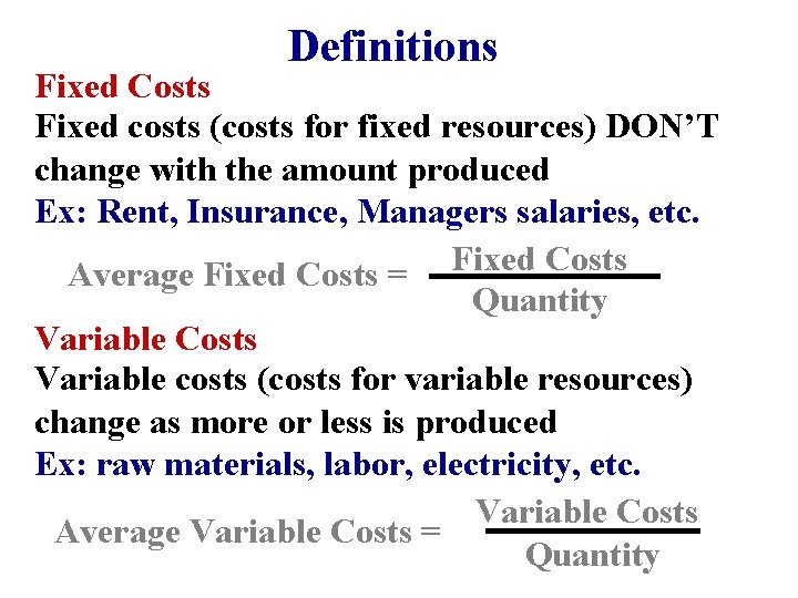
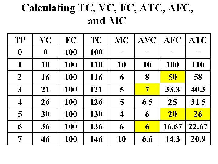
Definitions Fixed Costs Fixed costs (costs for fixed resources) DON’T change with the amount produced Ex: Rent, Insurance, Managers salaries, etc. Average Fixed Costs = Fixed Costs Quantity Variable Costs Variable costs (costs for variable resources) change as more or less is produced Ex: raw materials, labor, electricity, etc. Variable Costs Average Variable Costs = Quantity

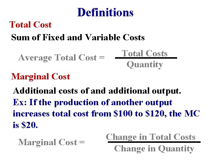
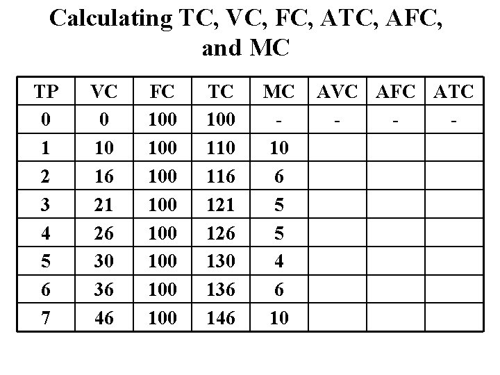
Definitions Total Cost Sum of Fixed and Variable Costs Average Total Cost = Total Costs Quantity Marginal Cost Additional costs of and additional output. Ex: If the production of another output increases total cost from $100 to $120, the MC is $20. Change in Total Costs Marginal Cost = Change in Quantity

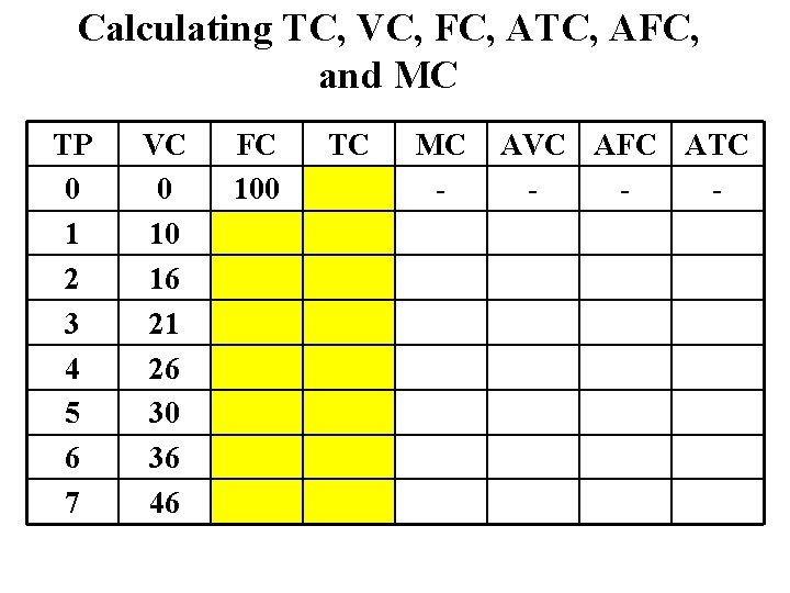
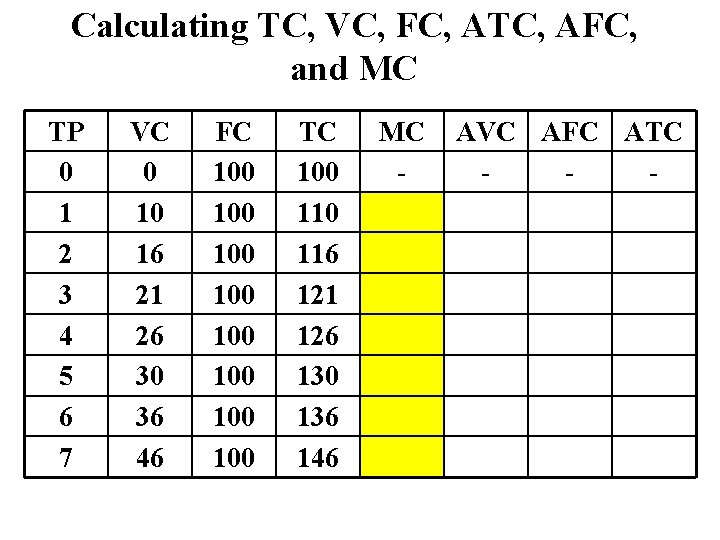
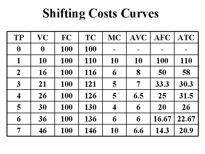
Calculating TC, VC, FC, ATC, AFC, and MC TP 0 1 2 3 4 5 6 7 VC 0 10 16 21 26 30 36 46 FC 100 TC MC - AVC AFC ATC -

Calculating TC, VC, FC, ATC, AFC, and MC TP 0 1 2 3 4 5 6 7 VC 0 10 16 21 26 30 36 46 FC 100 100 TC 100 116 121 126 130 136 146 MC - AVC AFC ATC -

Calculating TC, VC, FC, ATC, AFC, and MC TP 0 1 2 3 4 5 6 7 VC 0 10 16 21 26 30 36 46 FC 100 100 TC 100 116 121 126 130 136 146 MC 10 6 5 5 4 6 10 AVC AFC ATC -

Calculating TC, VC, FC, ATC, AFC, and MC TP 0 1 2 3 4 5 6 7 VC 0 10 16 21 26 30 36 46 FC 100 100 TC 100 116 121 126 130 136 146 MC 10 6 5 5 4 6 10 AVC AFC ATC 10 100 110 8 58 33. 3 40. 3 6. 5 25 31. 5 6 16. 67 22. 67 6. 6 14. 3 20. 9

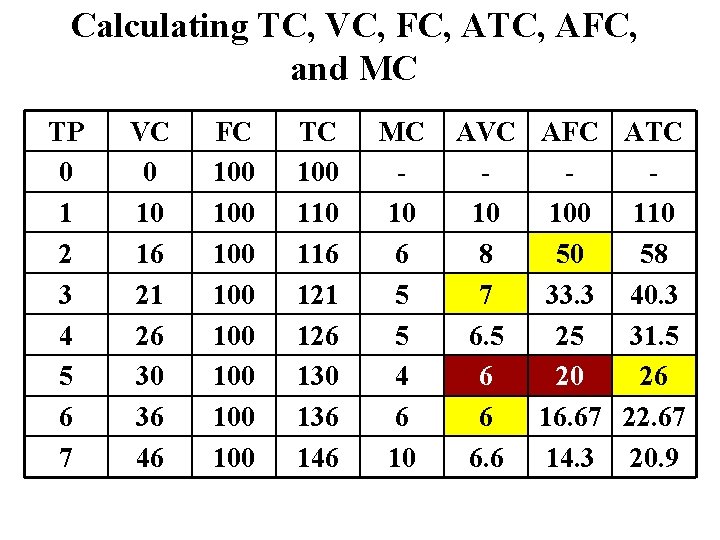
Calculating TC, VC, FC, ATC, AFC, and MC TP 0 1 2 3 4 5 6 7 VC 0 10 16 21 26 30 36 46 FC 100 100 TC 100 116 121 126 130 136 146 MC 10 6 5 5 4 6 10 AVC AFC ATC 10 100 110 8 50 58 7 33. 3 40. 3 6. 5 25 31. 5 6 20 26 6 16. 67 22. 67 6. 6 14. 3 20. 9

Calculating TC, VC, FC, ATC, AFC, and MC TP 0 1 2 3 4 5 6 7 VC 0 10 16 21 26 30 36 46 FC 100 100 TC 100 116 121 126 130 136 146 MC 10 6 5 5 4 6 10 AVC AFC ATC 10 100 110 8 50 58 7 33. 3 40. 3 6. 5 25 31. 5 6 20 26 6 16. 67 22. 67 6. 6 14. 3 20. 9

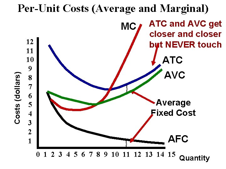
Per-Unit Costs (Average and Marginal) Costs (dollars) MC 12 11 10 9 8 7 6 5 4 3 2 1 ATC and AVC get closer and closer but NEVER touch ATC AVC Average Fixed Cost AFC 0 1 2 3 4 5 6 7 8 9 10 11 12 13 14 15 Quantity

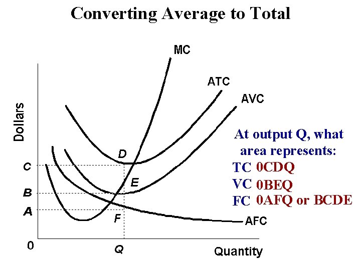
Converting Average to Total At output Q, what area represents: TC 0 CDQ VC 0 BEQ FC 0 AFQ or BCDE

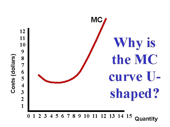
Costs (dollars) MC 12 11 10 9 8 7 6 5 4 3 2 1 Why is the MC curve Ushaped? 0 1 2 3 4 5 6 7 8 9 10 11 12 13 14 15 Quantity

Why is the MC curve U-shaped? • The MC curve falls and then rises because of diminishing marginal returns • The additional cost of the first units produced fall when workers have increasing marginal returns. • As production continues, each worker adds less and less to production so the marginal cost for each unit increases.

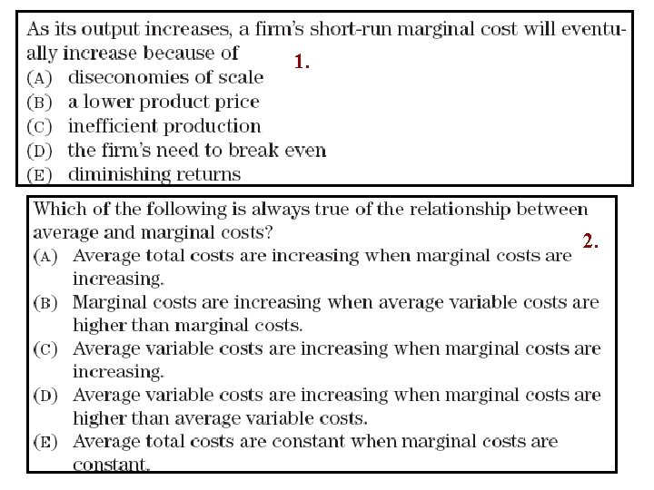
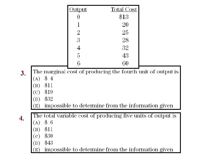
1. 2.

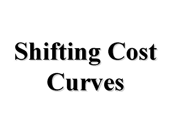
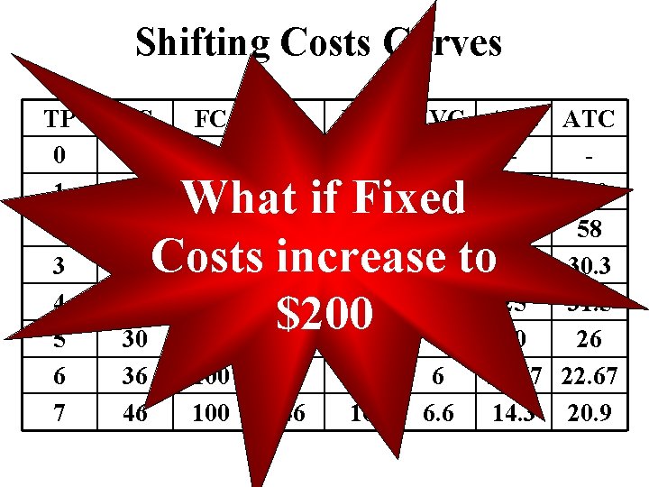
3. 4.

Shifting Cost Curves

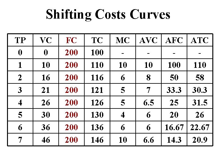
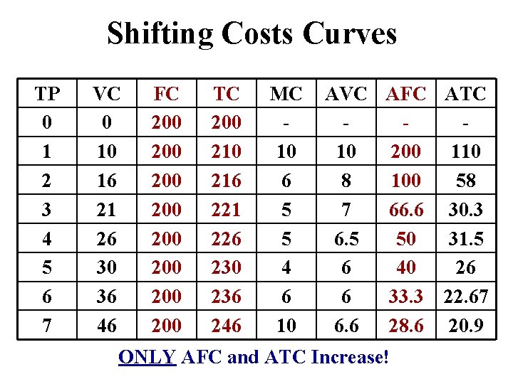
Shifting Costs Curves TP 0 1 2 3 4 5 6 7 VC 0 10 16 21 26 30 36 46 FC 100 100 TC 100 116 121 126 130 136 146 MC 10 6 5 3 4 6 10 AVC AFC ATC 10 100 110 8 50 58 7 33. 3 30. 3 6. 5 25 31. 5 6 20 26 6 16. 67 22. 67 6. 6 14. 3 20. 9 What if Fixed Costs increase to $200

Shifting Costs Curves TP 0 1 2 3 4 5 6 7 VC 0 10 16 21 26 30 36 46 FC 100 100 TC 100 116 121 126 130 136 146 MC 10 6 5 5 4 6 10 AVC AFC ATC 10 100 110 8 50 58 7 33. 3 30. 3 6. 5 25 31. 5 6 20 26 6 16. 67 22. 67 6. 6 14. 3 20. 9

Shifting Costs Curves TP 0 1 2 3 4 5 6 7 VC 0 10 16 21 26 30 36 46 FC 200 200 TC 100 116 121 126 130 136 146 MC 10 6 5 5 4 6 10 AVC AFC ATC 10 100 110 8 50 58 7 33. 3 30. 3 6. 5 25 31. 5 6 20 26 6 16. 67 22. 67 6. 6 14. 3 20. 9

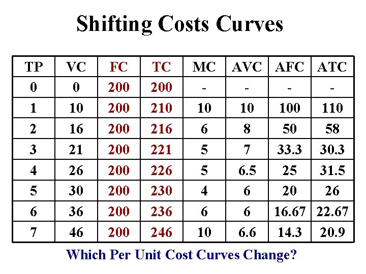
Shifting Costs Curves TP 0 1 2 3 4 5 6 7 VC 0 10 16 21 26 30 36 46 FC 200 200 TC 200 216 221 226 230 236 246 MC 10 6 5 5 4 6 10 AVC AFC ATC 10 100 110 8 50 58 7 33. 3 30. 3 6. 5 25 31. 5 6 20 26 6 16. 67 22. 67 6. 6 14. 3 20. 9 Which Per Unit Cost Curves Change?

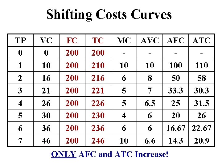
Shifting Costs Curves TP 0 1 2 3 4 5 6 7 VC 0 10 16 21 26 30 36 46 FC 200 200 TC 200 216 221 226 230 236 246 MC 10 6 5 5 4 6 10 AVC AFC ATC 10 100 110 8 50 58 7 33. 3 30. 3 6. 5 25 31. 5 6 20 26 6 16. 67 22. 67 6. 6 14. 3 20. 9 ONLY AFC and ATC Increase!

Shifting Costs Curves TP 0 1 2 3 4 5 6 7 VC 0 10 16 21 26 30 36 46 FC 200 200 TC 200 216 221 226 230 236 246 MC 10 6 5 5 4 6 10 AVC AFC ATC 10 200 110 8 100 58 7 66. 6 30. 3 6. 5 50 31. 5 6 40 26 6 33. 3 22. 67 6. 6 28. 6 20. 9 ONLY AFC and ATC Increase!

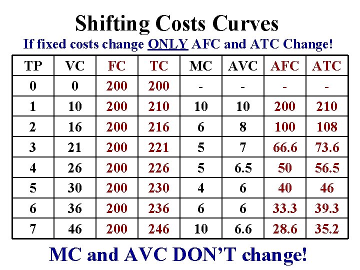
Shifting Costs Curves If fixed costs change ONLY AFC and ATC Change! TP 0 1 2 3 4 5 6 7 VC 0 10 16 21 26 30 36 46 FC 200 200 TC 200 216 221 226 230 236 246 MC 10 6 5 5 4 6 10 AVC AFC ATC 10 200 210 8 100 108 7 66. 6 73. 6 6. 5 50 56. 5 6 40 46 6 33. 3 39. 3 6. 6 28. 6 35. 2 MC and AVC DON’T change!

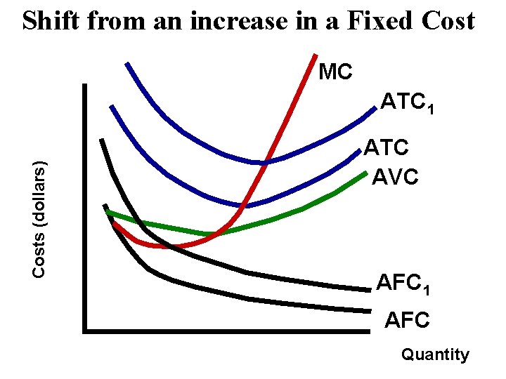
Shift from an increase in a Fixed Cost MC Costs (dollars) ATC 1 ATC AVC AFC 1 AFC Quantity

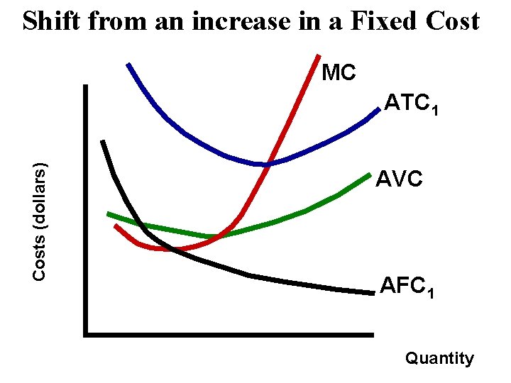
Shift from an increase in a Fixed Cost MC Costs (dollars) ATC 1 AVC AFC 1 Quantity

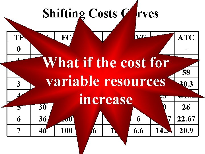
Shifting Costs Curves TP 0 1 2 3 4 5 6 7 VC 0 10 16 21 26 30 36 46 FC 100 100 TC 100 116 121 126 130 136 146 MC 10 6 5 5 4 6 10 AVC AFC ATC 10 100 110 8 50 58 7 33. 3 30. 3 6. 5 25 31. 5 6 20 26 6 16. 67 22. 67 6. 6 14. 3 20. 9 What if the cost for variable resources increase

Shifting Costs Curves TP 0 1 2 3 4 5 6 7 VC 0 10 16 21 26 30 36 46 FC 100 100 TC 100 116 121 126 130 136 146 MC 10 6 5 5 4 6 10 AVC AFC ATC 10 100 110 8 50 58 7 33. 3 30. 3 6. 5 25 31. 5 6 20 26 6 16. 67 22. 67 6. 6 14. 3 20. 9

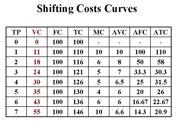
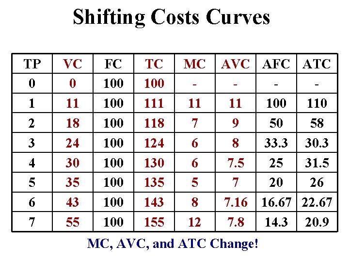
Shifting Costs Curves TP 0 1 2 3 4 5 6 7 VC 0 11 18 24 30 35 43 55 FC 100 100 TC 100 116 121 126 130 136 146 MC 10 6 5 5 4 6 10 AVC AFC ATC 10 100 110 8 50 58 7 33. 3 30. 3 6. 5 25 31. 5 6 20 26 6 16. 67 22. 67 6. 6 14. 3 20. 9

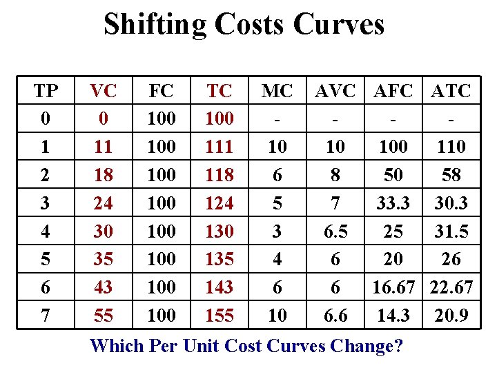
Shifting Costs Curves TP 0 1 2 3 4 5 6 7 VC 0 11 18 24 30 35 43 55 FC 100 100 TC 100 111 118 124 130 135 143 155 MC 10 6 5 3 4 6 10 AVC AFC ATC 10 100 110 8 50 58 7 33. 3 30. 3 6. 5 25 31. 5 6 20 26 6 16. 67 22. 67 6. 6 14. 3 20. 9 Which Per Unit Cost Curves Change?

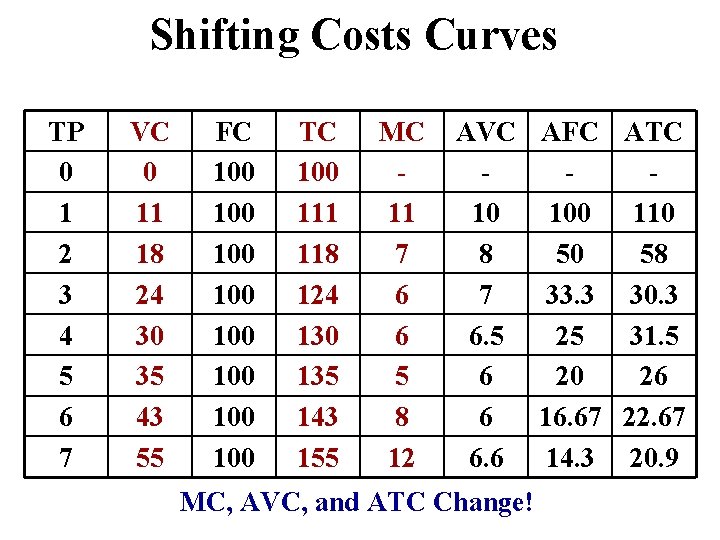
Shifting Costs Curves TP 0 1 2 3 4 5 6 7 VC 0 11 18 24 30 35 43 55 FC 100 100 TC 100 111 118 124 130 135 143 155 MC 11 7 6 6 5 8 12 AVC AFC ATC 10 100 110 8 50 58 7 33. 3 30. 3 6. 5 25 31. 5 6 20 26 6 16. 67 22. 67 6. 6 14. 3 20. 9 MC, AVC, and ATC Change!

Shifting Costs Curves TP 0 1 2 3 4 5 6 7 VC 0 11 18 24 30 35 43 55 FC 100 100 TC 100 111 118 124 130 135 143 155 MC 11 7 6 6 5 8 12 AVC AFC ATC 11 100 110 9 50 58 8 33. 3 30. 3 7. 5 25 31. 5 7 20 26 7. 16 16. 67 22. 67 7. 8 14. 3 20. 9 MC, AVC, and ATC Change!

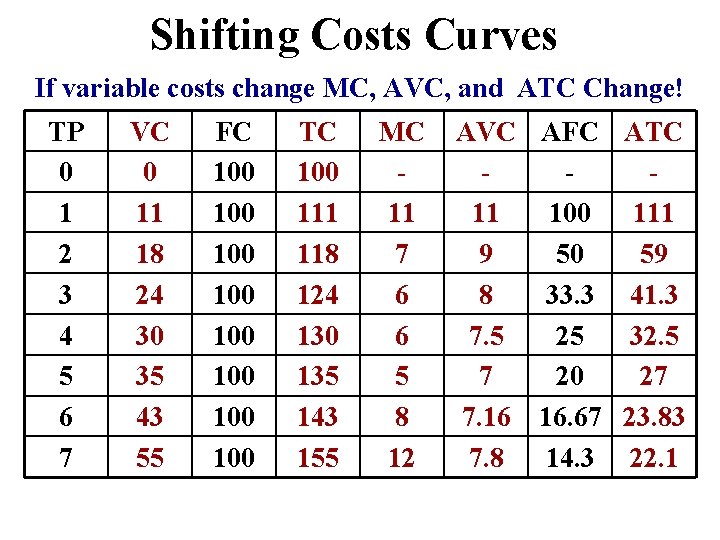
Shifting Costs Curves If variable costs change MC, AVC, and ATC Change! TP 0 1 2 3 4 5 6 7 VC 0 11 18 24 30 35 43 55 FC 100 100 TC 100 111 118 124 130 135 143 155 MC 11 7 6 6 5 8 12 AVC AFC ATC 11 100 111 9 50 59 8 33. 3 41. 3 7. 5 25 32. 5 7 20 27 7. 16 16. 67 23. 83 7. 8 14. 3 22. 1

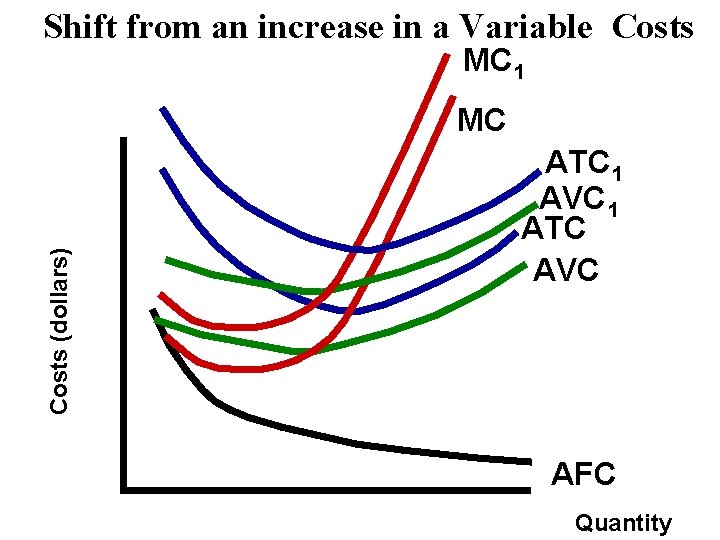
Shift from an increase in a Variable Costs MC 1 Costs (dollars) MC ATC 1 AVC 1 ATC AVC AFC Quantity

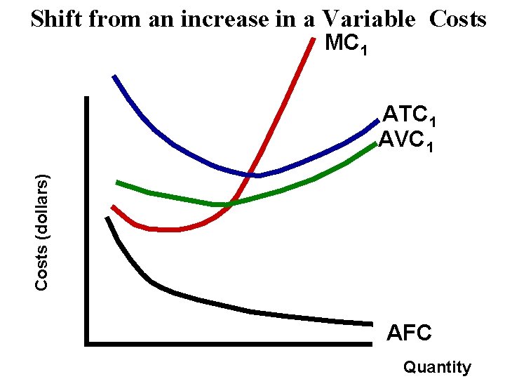
Shift from an increase in a Variable Costs MC 1 Costs (dollars) ATC 1 AVC 1 AFC Quantity

Long-Run Cost Curves

Short-Run vs. Long-Run • The short-run is a period in which at least one resource is fixed. – Plant capacity/size is NOT changeable • In the long-run ALL resources are variable – NO fixed resources – Plant capacity/size is changeable

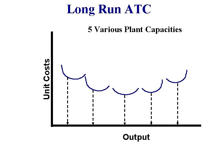
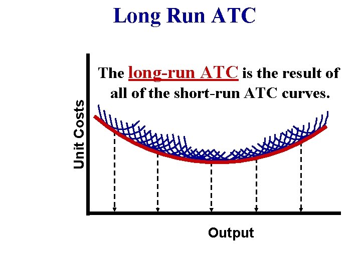
Long Run ATC What happens to the average total costs of a product when a firm increases its plant capacity? Example of various plant sizes: • I make looms out of my garage with one saw • I rent out building, buy 5 saws, hire 3 workers • I rent a factory, buy 20 saws and hire 40 workers • I build my own plant and use robots to build looms. • I create plants in every major city in the U. S. Long Run ATC curve is made up of all the different short run ATC curves of various plant sizes.

Long Run ATC Unit Costs 5 Various Plant Capacities Output

Unit Costs Long Run ATC The long-run ATC is the result of all of the short-run ATC curves. Output

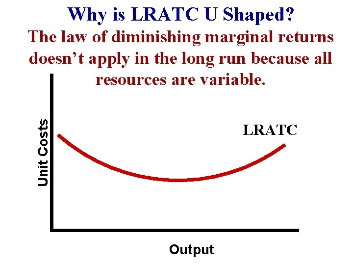
Why is LRATC U Shaped? Unit Costs The law of diminishing marginal returns doesn’t apply in the long run because all resources are variable. LRATC Output

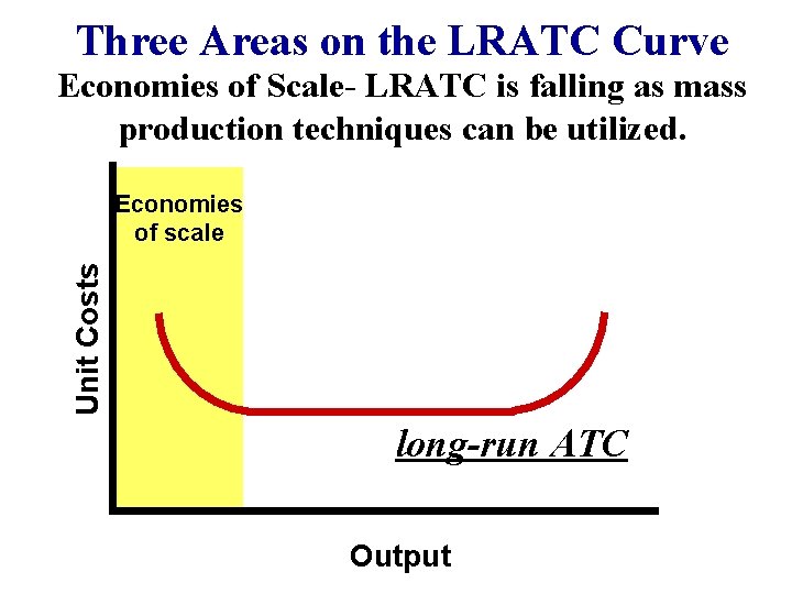
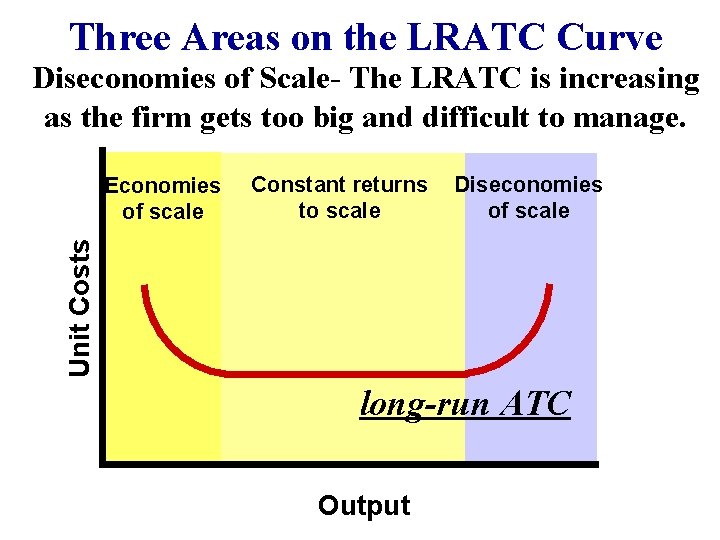
Three Areas on the LRATC Curve Economies of Scale- LRATC is falling as mass production techniques can be utilized. Unit Costs Economies of scale long-run ATC Output

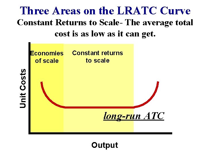
Three Areas on the LRATC Curve Constant Returns to Scale- The average total cost is as low as it can get. Constant returns to scale Unit Costs Economies of scale long-run ATC Output

Three Areas on the LRATC Curve Diseconomies of Scale- The LRATC is increasing as the firm gets too big and difficult to manage. Constant returns to scale Diseconomies of scale Unit Costs Economies of scale long-run ATC Output

Perfect Competition

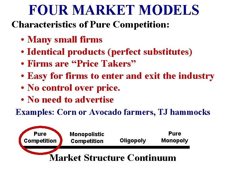
FOUR MARKET MODELS Characteristics of Pure Competition: • Many small firms • Identical products (perfect substitutes) • Firms are “Price Takers” • Easy for firms to enter and exit the industry • No control over price. • No need to advertise Examples: Corn or Avocado farmers, TJ hammocks Pure Competition Monopolistic Competition Oligopoly Pure Monopoly Market Structure Continuum

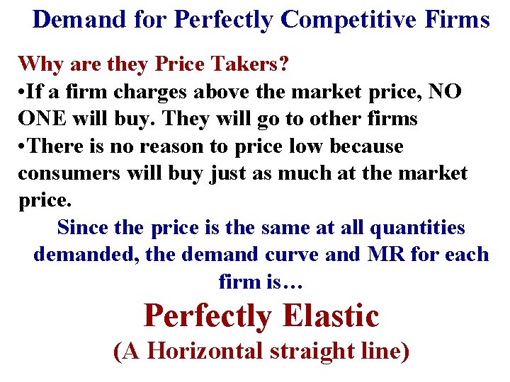
Demand for Perfectly Competitive Firms Why are they Price Takers? • If a firm charges above the market price, NO ONE will buy. They will go to other firms • There is no reason to price low because consumers will buy just as much at the market price. Since the price is the same at all quantities demanded, the demand curve and MR for each firm is… Perfectly Elastic (A Horizontal straight line)

Maximizing PROFIT

Maximizing PROFIT Profit Maximizing Rule MR = MC

Draw a FIRM making a profit

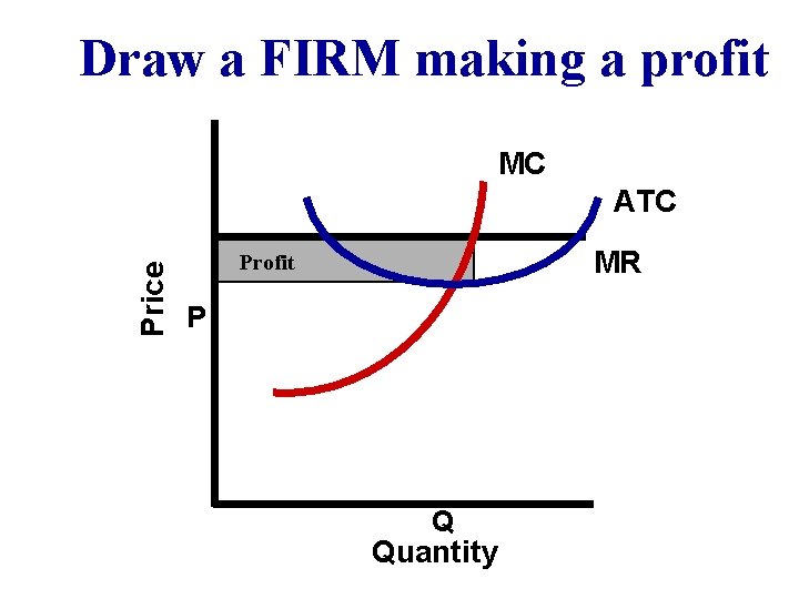
Draw a FIRM making a profit MC Price ATC MR Profit P Q Quantity

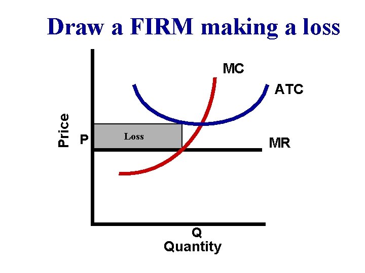
Draw a FIRM making a loss

Draw a FIRM making a loss MC Price ATC P Loss MR Q Quantity

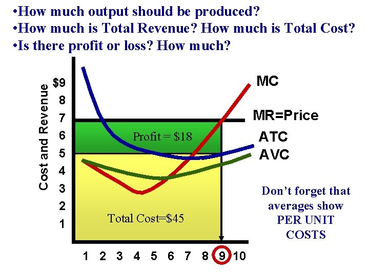
Cost and Revenue • How much output should be produced? • How much is Total Revenue? How much is Total Cost? • Is there profit or loss? How much? $9 8 7 6 5 4 3 2 1 MC Profit = $18 Total Cost=$45 Total Revenue =$63 1 2 3 4 5 6 7 8 9 10 MR=Price ATC AVC Don’t forget that averages show PER UNIT COSTS

Loss Minimization Position What would happen if the price is lowered from $7 to $5… the MR=MC rule still applies …but the output changes.

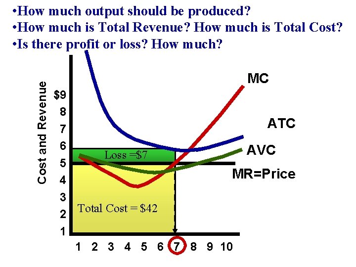
Cost and Revenue • How much output should be produced? • How much is Total Revenue? How much is Total Cost? • Is there profit or loss? How much? MC $9 8 ATC 7 6 AVC Loss =$7 5 MR=Price 4 3 Total Cost = $42 2 Total Revenue=$35 1 1 2 3 4 5 6 7 8 9 10

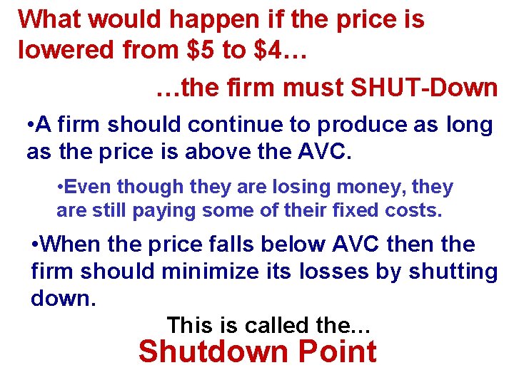
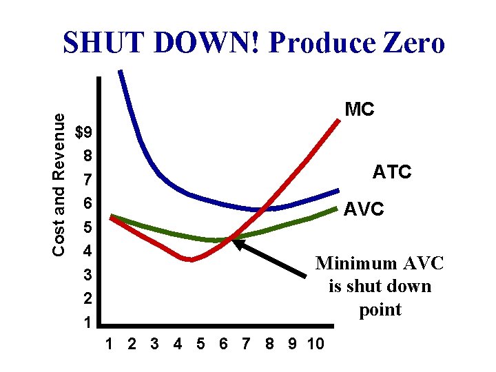
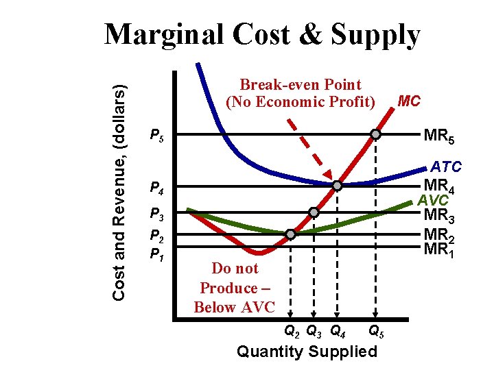
What would happen if the price is lowered from $5 to $4… …the firm must SHUT-Down • A firm should continue to produce as long as the price is above the AVC. • Even though they are losing money, they are still paying some of their fixed costs. • When the price falls below AVC then the firm should minimize its losses by shutting down. This is called the… Shutdown Point

Cost and Revenue SHUT DOWN! Produce Zero MC $9 8 7 6 5 4 3 2 1 ATC AVC Minimum AVC is shut down point 1 2 3 4 5 6 7 8 9 10

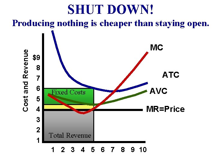
SHUT DOWN! Cost and Revenue Producing nothing is cheaper than staying open. MC $9 8 7 6 5 4 3 2 1 ATC AVC Fixed Costs MR=Price Total Cost Total Revenue 1 2 3 4 5 6 7 8 9 10

Supply Revisited

Cost and Revenue, (dollars) Marginal Cost & Supply Break-even Point (No Economic Profit) MC MR 5 P 5 ATC MR 4 P 4 AVC MR 3 MR 2 MR 1 P 3 P 2 P 1 Do not Produce – Below AVC Q 2 Q 3 Q 4 Q 5 Quantity Supplied

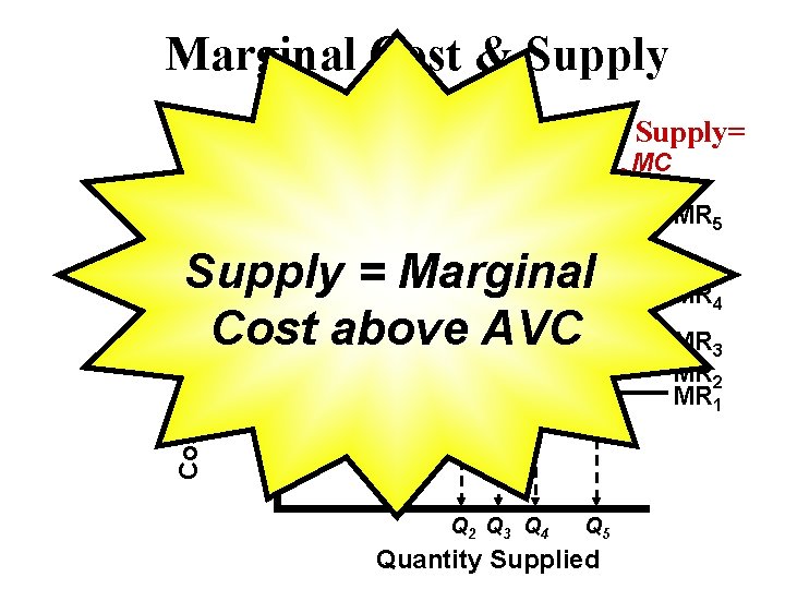
Cost and Revenue, (dollars) Marginal Cost & Supply This is the Supply Curve Supply= MC MR 5 P 5 Supply = Marginal P Cost above AVC P 4 3 P 2 P 1 Q 2 Q 3 Q 4 Q 5 Quantity Supplied MR 4 MR 3 MR 2 MR 1

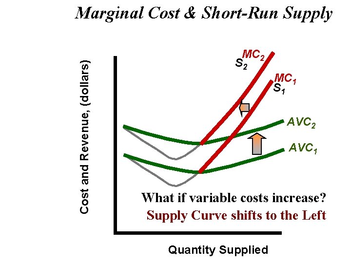
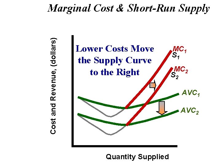
Cost and Revenue, (dollars) Marginal Cost & Short-Run Supply MC 2 S 2 MC 1 S 1 AVC 2 AVC 1 What if variable costs increase? Supply Curve shifts to the Left Quantity Supplied

Cost and Revenue, (dollars) Marginal Cost & Short-Run Supply Lower Costs Move the Supply Curve to the Right MC 1 S 1 MC 2 S 2 AVC 1 AVC 2 Quantity Supplied

Perfect Competition in the Long-Run

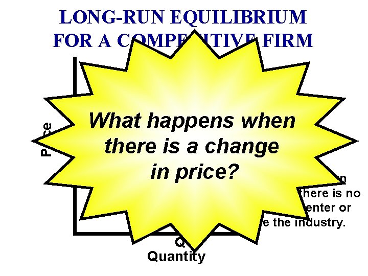
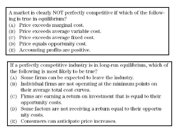
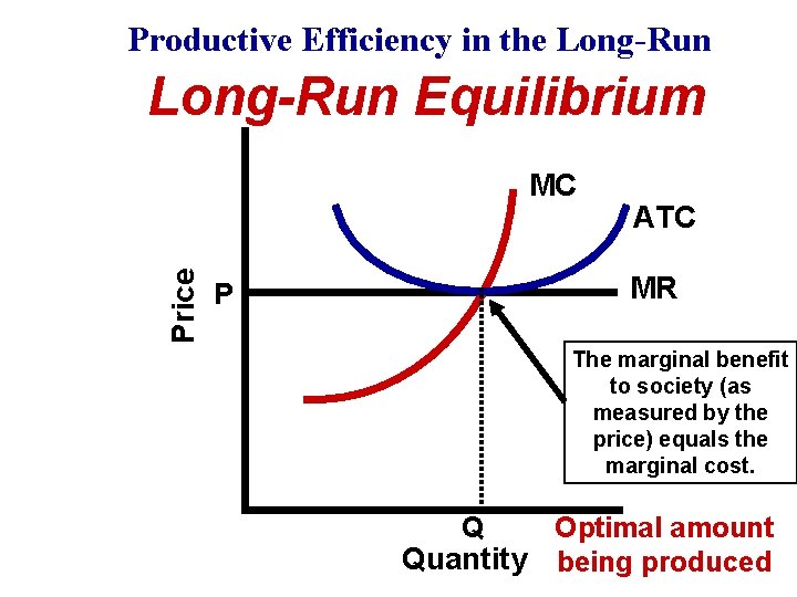
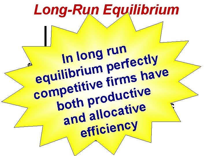
In the Long-run… • Firms will enter if there is profit • Firms will leave if there is loss • All firms break even, they make NO economic profit (No Economic Profit=Normal Profit) • In long run equilibrium the firm is efficient. (Price = Minimum ATC)

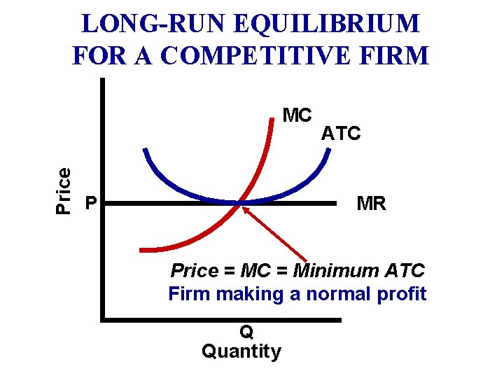
LONG-RUN EQUILIBRIUM FOR A COMPETITIVE FIRM Price MC ATC MR P Price = MC = Minimum ATC Firm making a normal profit Q Quantity

LONG-RUN EQUILIBRIUM FOR A COMPETITIVE FIRM Price MC P ATC What happens when there is a change MR in price? When at Long-Run Equilibrium, there is no incentive to enter or leave the industry. Q Quantity

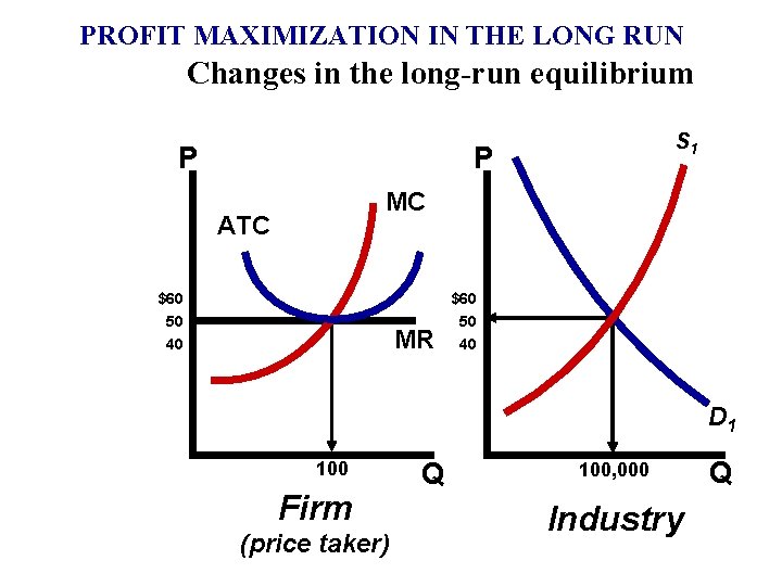
PROFIT MAXIMIZATION IN THE LONG RUN Changes in the long-run equilibrium P S 1 P MC ATC $60 50 40 MR D 1 100 Firm (price taker) Q 100, 000 Industry Q

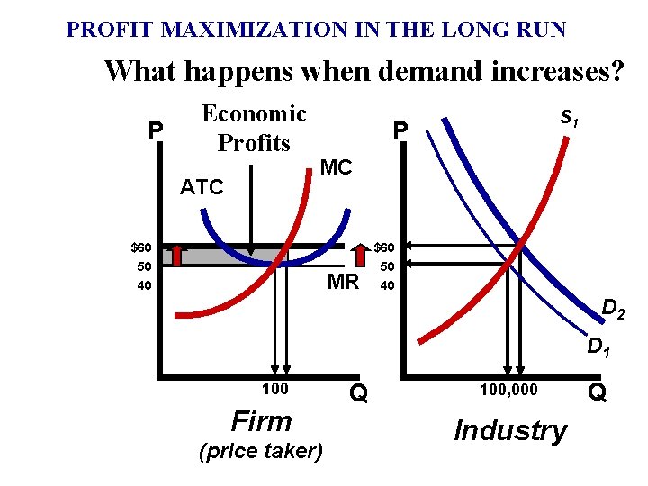
PROFIT MAXIMIZATION IN THE LONG RUN What happens when demand increases? P Economic Profits ATC S 1 P MC $60 50 40 MR D 2 D 1 100 Firm (price taker) Q 100, 000 Industry Q

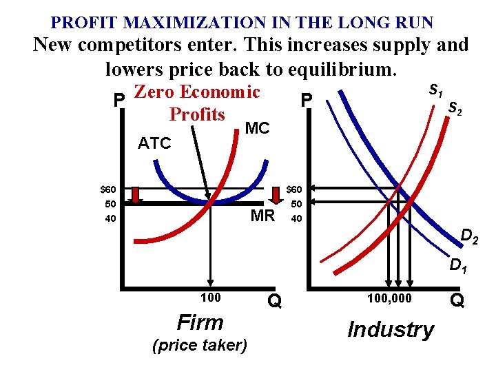
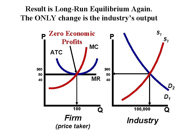
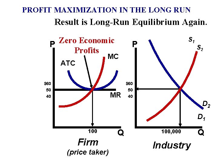
PROFIT MAXIMIZATION IN THE LONG RUN New competitors enter. This increases supply and lowers price back to equilibrium. P Zero Economic Profits S 1 P S 2 MC ATC $60 50 40 MR D 2 D 1 100 Firm (price taker) Q 100, 000 Industry Q

Result is Long-Run Equilibrium Again. The ONLY change is the industry’s output P Zero Economic Profits S 1 P S 2 MC ATC $60 50 40 MR D 2 D 1 100 Firm (price taker) Q 100, 000 Industry Q

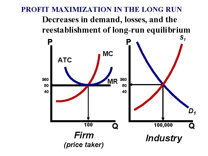
PROFIT MAXIMIZATION IN THE LONG RUN Decreases in demand, losses, and the reestablishment of long-run equilibrium P S 1 P MC ATC $60 MR $60 50 50 40 40 D 1 100 Firm (price taker) Q 100, 000 Industry Q

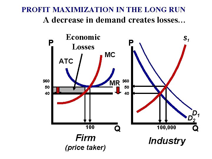
PROFIT MAXIMIZATION IN THE LONG RUN A decrease in demand creates losses… P Economic Losses ATC S 1 P MC $60 MR $60 50 50 40 40 D 1 D 2 100 Firm (price taker) Q 100, 000 Industry Q

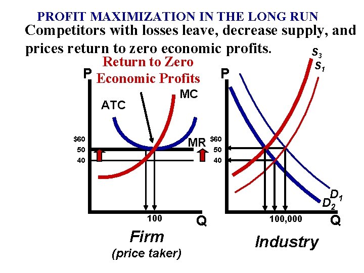
PROFIT MAXIMIZATION IN THE LONG RUN Competitors with losses leave, decrease supply, and prices return to zero economic profits. S 3 Return to Zero P Economic Profits S 1 P MC ATC $60 MR $60 50 50 40 40 D 1 D 2 100 Firm (price taker) Q 100, 000 Industry Q

PROFIT MAXIMIZATION IN THE LONG RUN Result is Long-Run Equilibrium Again. P Zero Economic Profits S 1 P S 2 MC ATC $60 50 40 MR D 2 D 1 100 Firm (price taker) Q 100, 000 Industry Q

Efficiency

PURE COMPETITION AND EFFICIENCY In general, efficiency is the optimal use of societies scarce resources • Perfect Competition forces producers to use limited resources to their fullest. • Inefficient firms have higher costs and are the first to leave the industry. • Perfectly competitive industries are extremely efficient There are two kinds of efficiency: 1. Productive Efficiency 2. Allocative Efficiency

PURE COMPETITION AND EFFICIENCY Productive Efficiency The production of a good in a least costly way. (Minimum amount of resources are being used) Graphically it is where… Price = Minimum ATC

PURE COMPETITION AND EFFICIENCY Allocative Efficiency The distribution of resources towards the production of products most wanted by society. Graphically it is where… Price(Marginal Benefit) = MC

Productive Efficiency in the Long-Run Equilibrium Price MC ATC MR P The marginal benefit to society (as measured by the price) equals the marginal cost. Optimal amount Quantity being produced Q

Long-Run Equilibrium Price MC ATC n u r g n y In lo l t c e f r e p m u MR i r e b v i l a i P h s equ m r i f e v i t e p e v m i t o c c u d o r p h t P = Minimumv. ATC = MC o b e i t a c o l l a and y c n e Qi c i f f e. Quantity