Short Run Equilibrium In Perfect Competition Lecture 19

Now What?

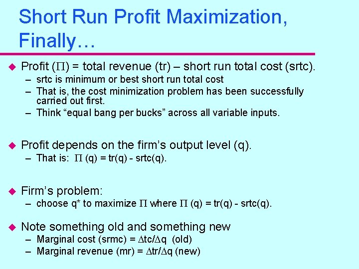
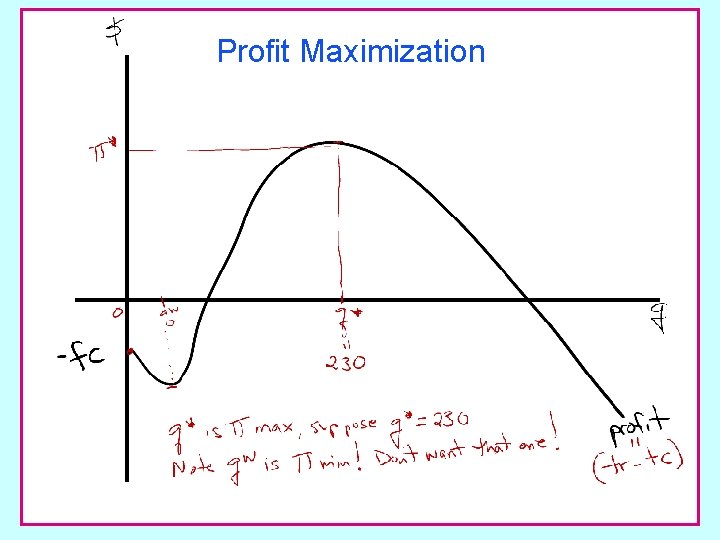
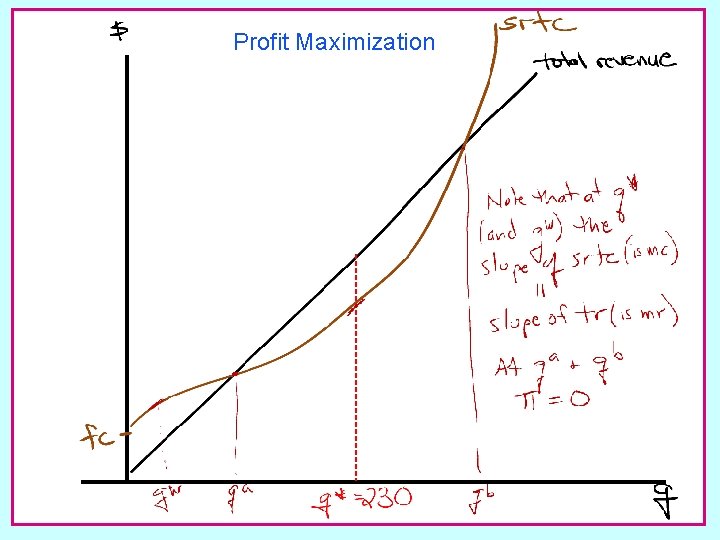
Short Run Profit Maximization, Finally… u Profit ( ) = total revenue (tr) – short run total cost (srtc). – srtc is minimum or best short run total cost – That is, the cost minimization problem has been successfully carried out first. – Think “equal bang per bucks” across all variable inputs. u Profit depends on the firm’s output level (q). – That is: (q) = tr(q) - srtc(q). u Firm’s problem: – choose q* to maximize where (q) = tr(q) - srtc(q). u Note something old and something new – Marginal cost (srmc) = tc/ q (old) – Marginal revenue (mr) = tr/ q (new)

Profit Maximization

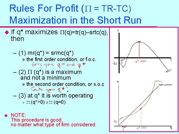
Rules For Profit ( = TR-TC) Maximization in the Short Run u If q* maximizes (q)=tr(q)–srtc(q), then – (1) mr(q*) = srmc(q*) » the first order condition, or f. o. c. – (2) (q*) is a maximum and not a minimum » the second order condition, or s. o. c – (3) at q* it is worth operating » u (q*>0) (q=0) NOTE: This procedure is good, no matter what type of firm considered.

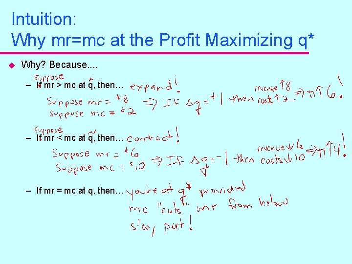
Intuition: Why mr=mc at the Profit Maximizing q* u Why? Because. . – If mr > mc at q, then… – If mr < mc at q, then… – If mr = mc at q, then…

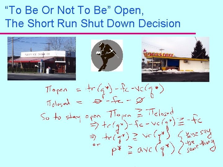
“To Be Or Not To Be” Open, The Short Run Shut Down Decision

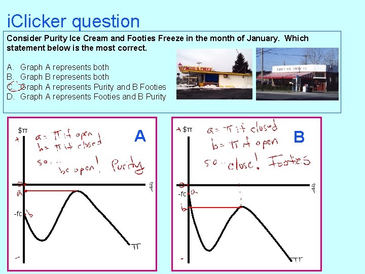
i. Clicker question Consider Purity Ice Cream and Footies Freeze in the month of January. Which statement below is the most correct. A. B. C. D. Graph A represents both Graph B represents both Graph A represents Purity and B Footies Graph A represents Footies and B Purity $π A $π -fc B

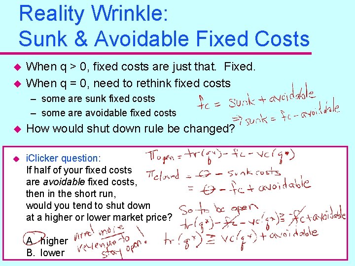
Reality Wrinkle: Sunk & Avoidable Fixed Costs u u When q > 0, fixed costs are just that. Fixed. When q = 0, need to rethink fixed costs – some are sunk fixed costs – some are avoidable fixed costs u How would shut down rule be changed? u i. Clicker question: If half of your fixed costs are avoidable fixed costs, then in the short run, would you tend to shut down at a higher or lower market price? A. higher B. lower

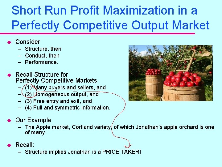
Short Run Profit Maximization in a Perfectly Competitive Output Market u Consider – Structure, then – Conduct, then – Performance. u Recall Structure for Perfectly Competitive Markets – – u (1) Many buyers and sellers, and (2) Homogeneous output, and (3) Free entry and exit, and (4) Full and symmetric information. Our Example – The Apple market, Cortland variety, of which Jonathan’s apple orchard is one of many u Recall: – Structure implies Jonathan is a PRICE TAKER!

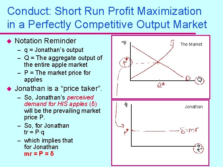
Conduct: Short Run Profit Maximization in a Perfectly Competitive Output Market u Notation Reminder – q = Jonathan’s output – Q = The aggregate output of the entire apple market – P = The market price for apples u The Market Jonathan is a “price taker”. – So, Jonathan’s perceived demand for HIS apples (δ) will be the prevailing market price P. – So, for Jonathan tr = P∙q – which implies that for Jonathan mr = P = δ Jonathan

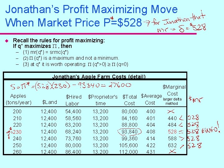
Jonathan’s Profit Maximizing Move When Market Price P=$528 u Recall the rules for profit maximizing: If q* maximizes , then – (1) mr(q*) = srmc(q*) – (2) (q*) is a maximum and not a minimum. – (3) at q* it is worth operating: (q*>0) (q=0) Jonathan's Apple Farm Costs (detail) Apples (tons/year) $Land 200 210 220 230 240 250 260 12, 400 12, 400 $Hired Labor 54, 400 58, 560 63, 200 68, 240 73, 760 80, 000 86, 400 $Proprietor's $Total Cost time 13, 200 80, 000 13, 200 84, 160 13, 200 88, 800 13, 200 93, 840 13, 200 99, 360 13, 200 105, 600 13, 200 112, 000 $Marginal $Average Cost larger delta method 400 401 404 408 414 422 431 440 484 528 588 632

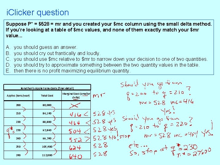
i. Clicker question Suppose P* = $528 = mr and you created your $mc column using the small delta method. If you’re looking at a table of $mc values, and none of them exactly match your $mr value. . . A. B. C. D. E. you should guess an answer. you should cry out frantically and loudly. you should use $mc relative to $mr to narrow down your decision to one of two quantities. you should try to approximate something between the two quantity values in the table. then there is no profit maximizing equilibrium quantity. Jonathan's Apple Farm Costs (finer detail) Apples (tons/year) Total Cost Marginal Cost (smaller delta) 200 80, 000 210 84, 160 220 88, 800 230 93, 840 240 99, 360 250 105, 600 260 112, 000

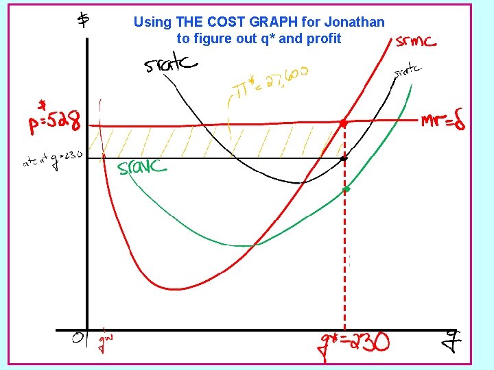
Using THE COST GRAPH for Jonathan to figure out q* and profit

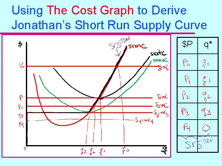
Using The Cost Graph to Derive Jonathan’s Short Run Supply Curve $P 0 q*

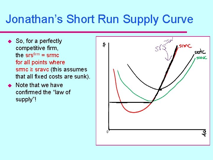
Jonathan’s Short Run Supply Curve u u So, for a perfectly competitive firm, the srsfirm = srmc for all points where srmc ≥ sravc (this assumes that all fixed costs are sunk). Note that we have confirmed the “law of supply”!

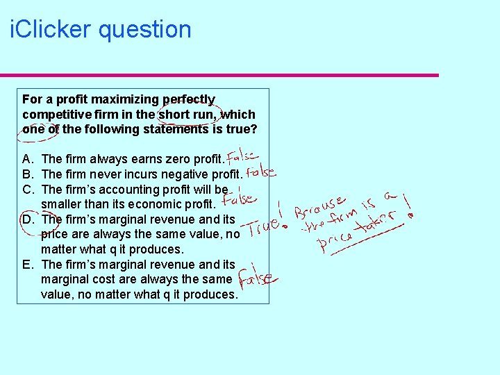
i. Clicker question For a profit maximizing perfectly competitive firm in the short run, which one of the following statements is true? A. The firm always earns zero profit. B. The firm never incurs negative profit. C. The firm’s accounting profit will be smaller than its economic profit. D. The firm’s marginal revenue and its price are always the same value, no matter what q it produces. E. The firm’s marginal revenue and its marginal cost are always the same value, no matter what q it produces.

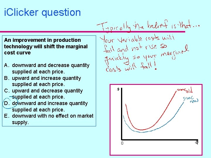
i. Clicker question An improvement in production technology will shift the marginal cost curve A. downward and decrease quantity supplied at each price. B. upward and increase quantity supplied at each price. C. upward and decrease quantity supplied at each price. D. downward and increase quantity supplied at each price. E. downward with no effect on market supply. 0

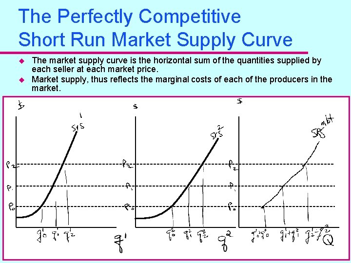
The Perfectly Competitive Short Run Market Supply Curve u u The market supply curve is the horizontal sum of the quantities supplied by each seller at each market price. Market supply, thus reflects the marginal costs of each of the producers in the market.

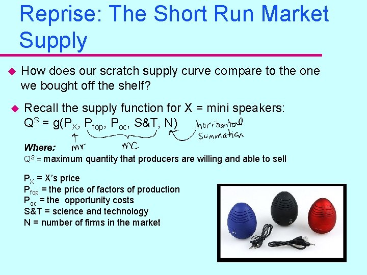
Reprise: The Short Run Market Supply u u How does our scratch supply curve compare to the one we bought off the shelf? Recall the supply function for X = mini speakers: QS = g(PX, Pfop, Poc, S&T, N) Where: QS = maximum quantity that producers are willing and able to sell PX = X’s price Pfop = the price of factors of production Poc = the opportunity costs S&T = science and technology N = number of firms in the market

Reprise: Producer’s Surplus – Again, Still u Recall that producer’s surplus measures the gain to the firm from selling all units at the market price. – PS on q units = Total Revenue – Variable Costs – PS on any particular unit = Price – Marginal Cost u We now know – Profit = Total Revenue – Variable Costs – Fixed Costs – Rearranging we get: » Variable Costs = Total Revenue – Fixed Costs – Profit – Plugging this expression for Variable Costs into PS we get: » PS on q units = Total Revenue – Total Revenue + Fixed Costs + Profit u So Producer’s Surplus can also be written as – PS on q units = Fixed Costs + Profit – An alternative interesting way to think of producer’s surplus u On the graph, Producer’s Surplus is – the area above the short run firm supply curve and below the market price

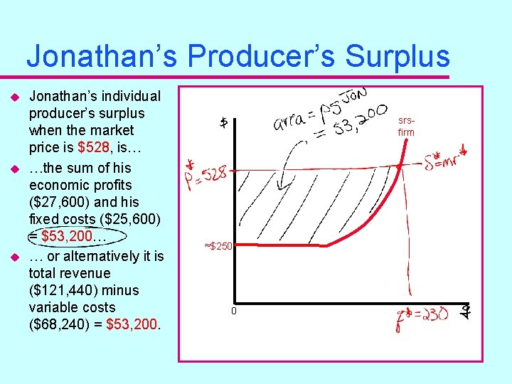
Jonathan’s Producer’s Surplus u u u Jonathan’s individual producer’s surplus when the market price is $528, is… …the sum of his economic profits ($27, 600) and his fixed costs ($25, 600) = $53, 200… … or alternatively it is total revenue ($121, 440) minus variable costs ($68, 240) = $53, 200. srsfirm ≈$250 0

SO: The Market & The Firm in Short Run Equilibrium u Given: – – u Market Demand Firms’ Technologies (including some fixed inputs) Factor Prices The Number of Firms Need: – Each firm is profit maximizing – Market Demand = Short Run Market Supply u Solve For: – – Q* q* P* profit*

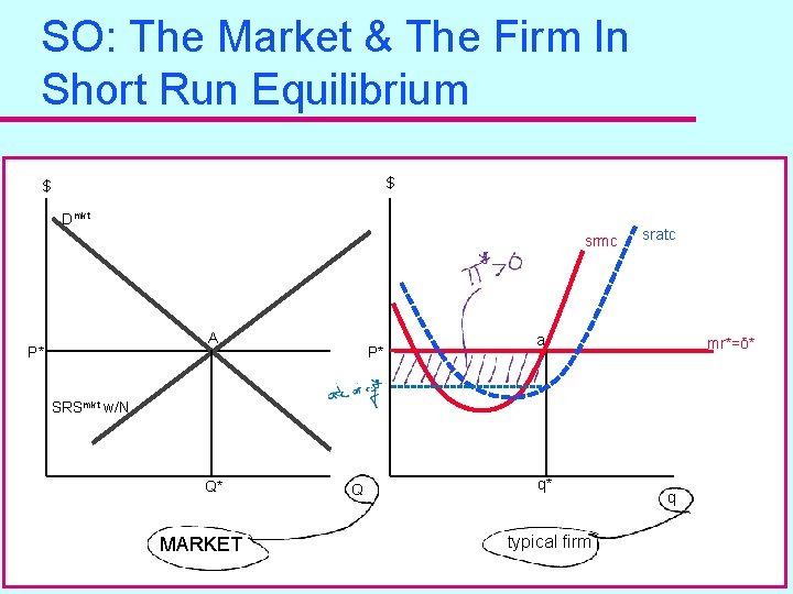
SO: The Market & The Firm In Short Run Equilibrium $ $ Dmkt srmc A P* P* sratc a mr*=δ* SRSmkt w/N Q* MARKET Q q* typical firm q

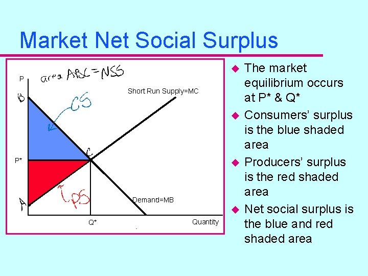
Market Net Social Surplus u P Short Run Supply=MC u P* u Demand=MB u Q* Quantity The market equilibrium occurs at P* & Q* Consumers’ surplus is the blue shaded area Producers’ surplus is the red shaded area Net social surplus is the blue and red shaded area