Perfect competition and pure monopoly Perfect competition the

Perfect competition and pure monopoly

Perfect competition – the competitive firm’s supply decision Part 1

Industries and the number of firms • An industry is the set of all firms making the same product. The output of an industry is the sum of the outputs of its firms. • Yet different industries have very different number of firms. Eurostar is the only supplier of train journeys from London to Paris. In contrast, the UK has hundreds of thousands of farms and tens of thousands of grocers. • Why do some industries have many firms but others only one? 3

Perfect competition and monopoly • First it is useful to establish two benchmark cases, extremes between which all other types of market structure must lie. These limiting cases are perfect competition and monopoly. • In a perfectly competitive market, both buyers and sellers believe that their own actions have no effect on the market price. • In contrast, a monopolist, the only seller or potential seller in the industry, sets the price. 4

Competitive demand • We focus on how the number of sellers affects the behaviour of sellers. • Buyers are in the background. We simply assume that there are many buyers whose individual downward-sloping demand curves can be aggregated into the market demand curve. • Thus, we assume that the demand side of the market is competitive, but contrast the different cases on the supply side. 5

Quantities demanded and supplied and perfect competition • Perfect competition means that each firm or household, recognizing that its quantities supplied or demanded are trivial relative to the whole market, assumes its actions have no effect on the market price. • This assumption was also built into our earlier model of consumer choice. Each consumer’s budget line took market prices as given, unaffected by the quantities then chosen. • Changes in market conditions, applying to all firms and consumers, change the equilibrium price and hence individual quantities demanded, but each consumer neglects any feedback from his own actions to market price. 6

Competition in theory and everyday usage • This concept of competition, which we now extend to firms and supply, differs from everyday usage. Ford and VW are fighting each other vigorously for the European car market, but an economist would not call them perfectly competitive. Each has such a big share of the market that changes in its quantity supplied affect the market price. • VW and Ford each take account of this in deciding how much to supply. They are not price-takers. • Only under perfect competition can individuals make decisions that treat the price as independent of their own actions. 7

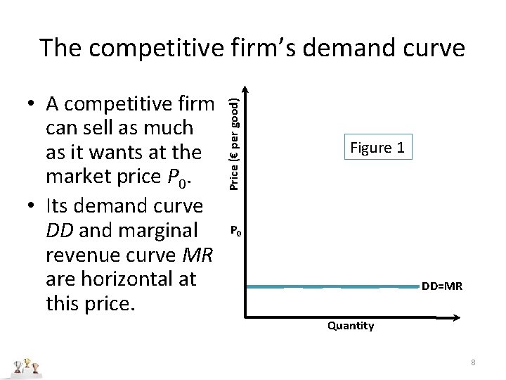
• A competitive firm can sell as much as it wants at the market price P 0. • Its demand curve DD and marginal revenue curve MR are horizontal at this price. Price (€ per good) The competitive firm’s demand curve Figure 1 P 0 DD=MR Quantity 8

Horizontal demand curve • If an individual’s action does not affect the price, a perfectly competitive industry must have many buyers and many sellers. • Each firm in a perfectly competitive industry faces a horizontal demand curve as in figure 1. • However much the firm sells, it gets the market price. If it charges a price above P 0 it will not sell any output: buyers will go to other firms whose product is just as good. Since the firm can sell as much as it wants at P 0, it will not charge less than P 0. The individual firm’s demand curve is DD. 9

Features of perfectly competitive firms • A horizontal demand curve is the key feature of a perfectly competitive firm. To be a plausible description of the demand curve facing the firm, the industry must have four attributes. • First, there must be many firms, each one trivial (= tiny) relative to the entire industry. • Second, the product must be standardized. 10

Homogeneous and heterogeneous products • Even if the car industry had many firms it would not be a perfectly competitive industry. • A Ford Mondeo is not a perfect substitute for an Opel Vectra. The more imperfect they are as substitutes, the more it makes sense to view Ford as the sole supplier of Mondeos and Opel (GM) as the sole supplier of Vectras. • Each producer then ceases to be trivial relative to the relevant market, and cannot act as a pricetaker. In a perfectly competitive industry, all firms must be making the same product, for which they all charge the same price. 11

Perfect and imperfect information • Even if all firms in an industry made homogeneous or identical goods, each firm may have some discretion over the price it charges if buyers have imperfect information about the quality or characteristics of products. • To rule this out in a competitive industry, we must assume that buyers have almost perfect information about the products being sold. They know the products of different firms in a competitive industry really are identical. 12

Free entry • Why don’t all the firms in the industry do what OPEC did in 1973 -74, collectively restricting supply, to increase the price of their output by moving the industry up its market demand curve? • The fourth crucial characteristic of a perfectly competitive industry is free entry and exit. Even if existing firms could organize themselves to restrict total supply and drive up the market price, the consequent rise in profits would simply attract new firms into the industry, thereby increasing total supply again and driving the price back down. 13

Free exit • Conversely, as we shall shortly see, when firms in a competitive industry are losing money, some firms will close down and, by reducing the number of firms remaining in the industry, reduce the total supply and drive the price up, thereby allowing the remaining firms to survive. 14

To sum up, each firm in a competitive industry faces a horizontal demand curve at the going market price. To be a plausible description of the demand conditions facing a firm, the industry must have: 1. many firms, each trivial relative to the industry; 2. a homogeneous product, so that buyers would switch between firms if their prices differed; 3. perfect customer information about product quality, so that buyers know that the products of different firms really are the same; and 4. free entry and exit, to remove any incentive for existing firms to collude. 15

The firm’s supply decision • Earlier, we developed a general theory of supply. • The firm uses the marginal condition (MC = MR) to find the best positive output; then it uses the average condition to check if the price for which this output is sold covers average cost. 16

The special case of perfectly competitive firms • This general theory must hold for the special case of perfectly competitive firms. • The special feature of perfect competition is the relationship between marginal revenue and price. • A competitive firm faces a horizontal demand curve. Making and selling extra output does not bid down the price for which existing output is sold. The extra revenue from selling an extra unit is simply the price received. • A perfectly competitive firm’s marginal revenue is its output price, MR = P (Eq. 1) 17

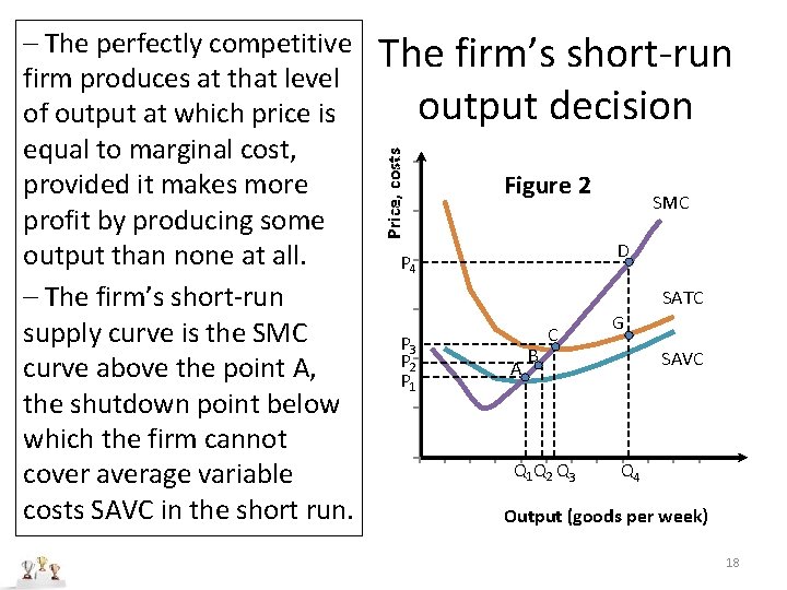
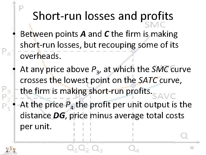
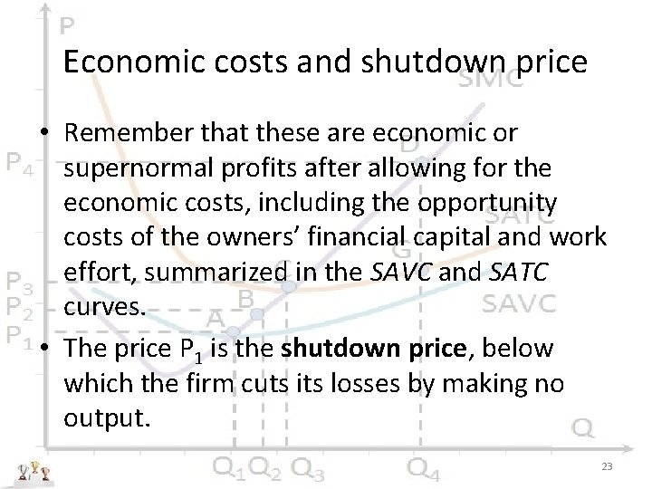
Price, costs – The perfectly competitive The firm’s short-run firm produces at that level output decision of output at which price is equal to marginal cost, 60 Figure 2 provided it makes more SMC 50 profit by producing some D output than none at all. 40 P 4 SATC – The firm’s short-run 30 G C supply curve is the SMC P 3 B SAVC 20 P 2 A curve above the point A, P 1 the shutdown point below 10 which the firm cannot 0 QQ Q Q cover average variable 0 1 2 3 41 52 63 7 8 4 9 10 11 week) costs SAVC in the short run. Output (goods per week) 18

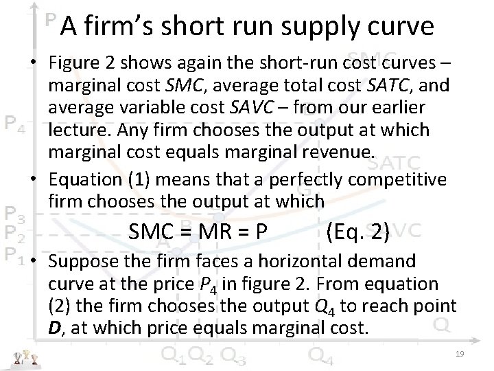
A firm’s short run supply curve • Figure 2 shows again the short-run cost curves – marginal cost SMC, average total cost SATC, and average variable cost SAVC – from our earlier lecture. Any firm chooses the output at which marginal cost equals marginal revenue. • Equation (1) means that a perfectly competitive firm chooses the output at which SMC = MR = P (Eq. 2) • Suppose the firm faces a horizontal demand curve at the price P 4 in figure 2. From equation (2) the firm chooses the output Q 4 to reach point D, at which price equals marginal cost. 19

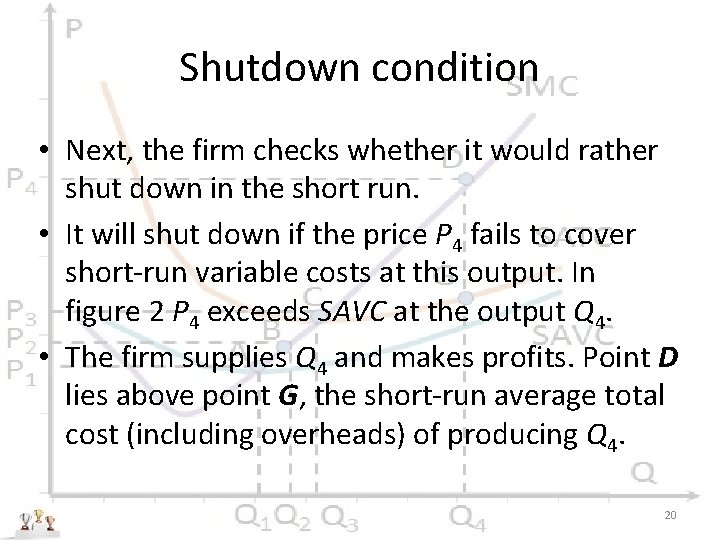
Shutdown condition • Next, the firm checks whether it would rather shut down in the short run. • It will shut down if the price P 4 fails to cover short-run variable costs at this output. In figure 2 P 4 exceeds SAVC at the output Q 4. • The firm supplies Q 4 and makes profits. Point D lies above point G, the short-run average total cost (including overheads) of producing Q 4. 20

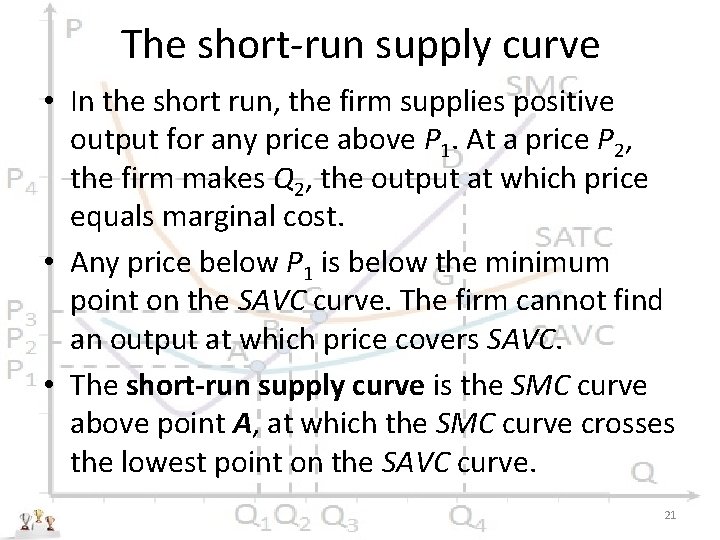
The short-run supply curve • In the short run, the firm supplies positive output for any price above P 1. At a price P 2, the firm makes Q 2, the output at which price equals marginal cost. • Any price below P 1 is below the minimum point on the SAVC curve. The firm cannot find an output at which price covers SAVC. • The short-run supply curve is the SMC curve above point A, at which the SMC curve crosses the lowest point on the SAVC curve. 21

Short-run losses and profits • Between points A and C the firm is making short-run losses, but recouping some of its overheads. • At any price above P 3, at which the SMC curve crosses the lowest point on the SATC curve, the firm is making short-run profits. • At the price P 4 the profit per unit output is the distance DG, price minus average total costs per unit. 22

Economic costs and shutdown price • Remember that these are economic or supernormal profits after allowing for the economic costs, including the opportunity costs of the owners’ financial capital and work effort, summarized in the SAVC and SATC curves. • The price P 1 is the shutdown price, below which the firm cuts its losses by making no output. 23

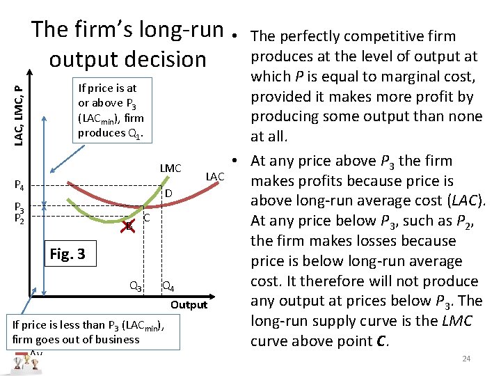
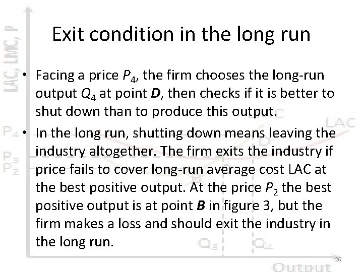
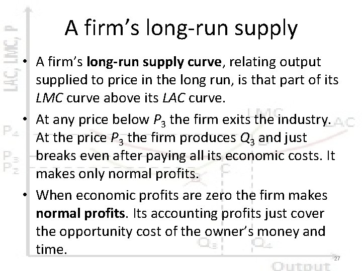
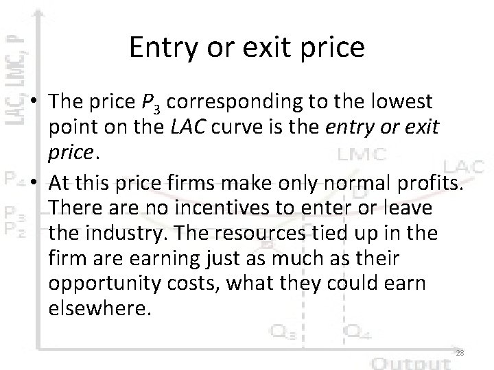
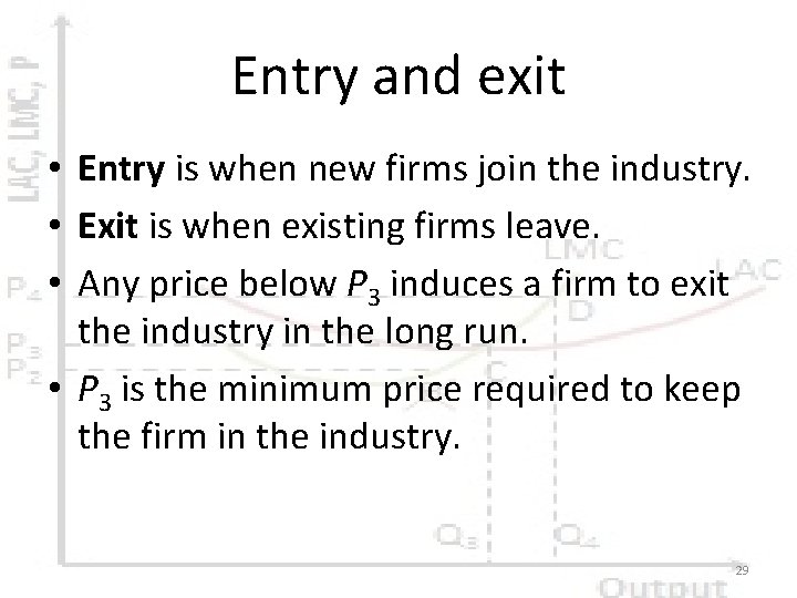
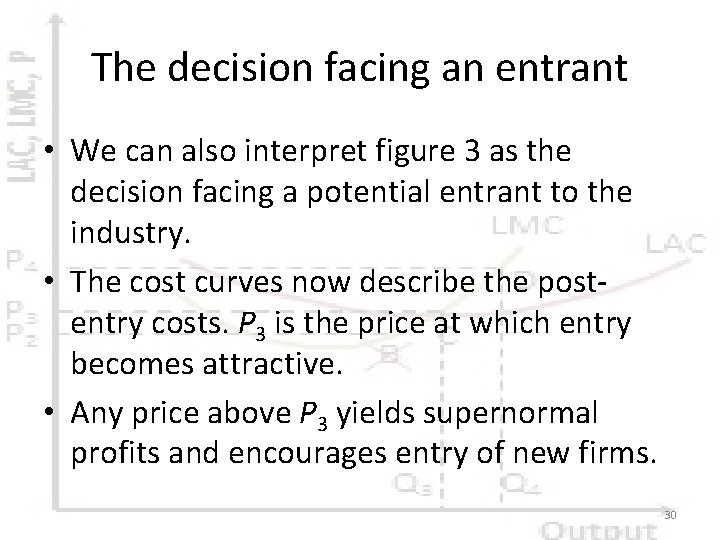
LAC, LMC, P The firm’s long-run • output decision If price is at or above P 3 (LACmin), firm produces Q 1. LMC P 4 LAC D P 3 P 2 B C Fig. 3 Q 4 Output If price is less than P 3 (LACmin), firm goes out of business Av. . . The perfectly competitive firm produces at the level of output at which P is equal to marginal cost, provided it makes more profit by producing some output than none at all. • At any price above P 3 the firm makes profits because price is above long-run average cost (LAC). At any price below P 3, such as P 2, the firm makes losses because price is below long-run average cost. It therefore will not produce any output at prices below P 3. The long-run supply curve is the LMC curve above point C. 24

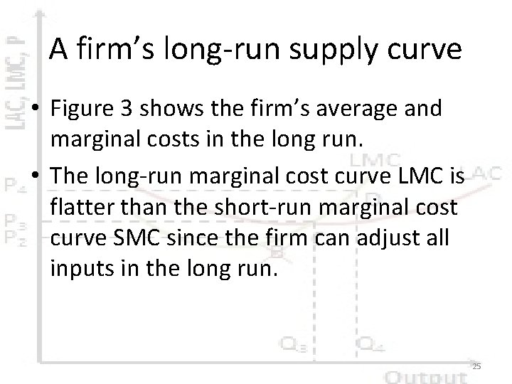
A firm’s long-run supply curve • Figure 3 shows the firm’s average and marginal costs in the long run. • The long-run marginal cost curve LMC is flatter than the short-run marginal cost curve SMC since the firm can adjust all inputs in the long run. 25

Exit condition in the long run • Facing a price P 4, the firm chooses the long-run output Q 4 at point D, then checks if it is better to shut down than to produce this output. • In the long run, shutting down means leaving the industry altogether. The firm exits the industry if price fails to cover long-run average cost LAC at the best positive output. At the price P 2 the best positive output is at point B in figure 3, but the firm makes a loss and should exit the industry in the long run. 26

A firm’s long-run supply • A firm’s long-run supply curve, relating output supplied to price in the long run, is that part of its LMC curve above its LAC curve. • At any price below P 3 the firm exits the industry. At the price P 3 the firm produces Q 3 and just breaks even after paying all its economic costs. It makes only normal profits. • When economic profits are zero the firm makes normal profits. Its accounting profits just cover the opportunity cost of the owner’s money and time. 27

Entry or exit price • The price P 3 corresponding to the lowest point on the LAC curve is the entry or exit price. • At this price firms make only normal profits. There are no incentives to enter or leave the industry. The resources tied up in the firm are earning just as much as their opportunity costs, what they could earn elsewhere. 28

Entry and exit • Entry is when new firms join the industry. • Exit is when existing firms leave. • Any price below P 3 induces a firm to exit the industry in the long run. • P 3 is the minimum price required to keep the firm in the industry. 29

The decision facing an entrant • We can also interpret figure 3 as the decision facing a potential entrant to the industry. • The cost curves now describe the postentry costs. P 3 is the price at which entry becomes attractive. • Any price above P 3 yields supernormal profits and encourages entry of new firms. 30

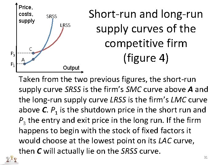
Price, costs, supply P 3 P 1 SRSS LRSS C A Output Short-run and long-run supply curves of the competitive firm (figure 4) Taken from the two previous figures, the short-run supply curve SRSS is the firm’s SMC curve above A and the long-run supply curve LRSS is the firm’s LMC curve above C. P 1 is the shutdown price in the short run and P 3 the entry and exit price in the long run. If the firm happens to begin with the stock of fixed factors it would choose at the lowest point on its LAC curve, then C will actually lie on the SRSS curve. 31

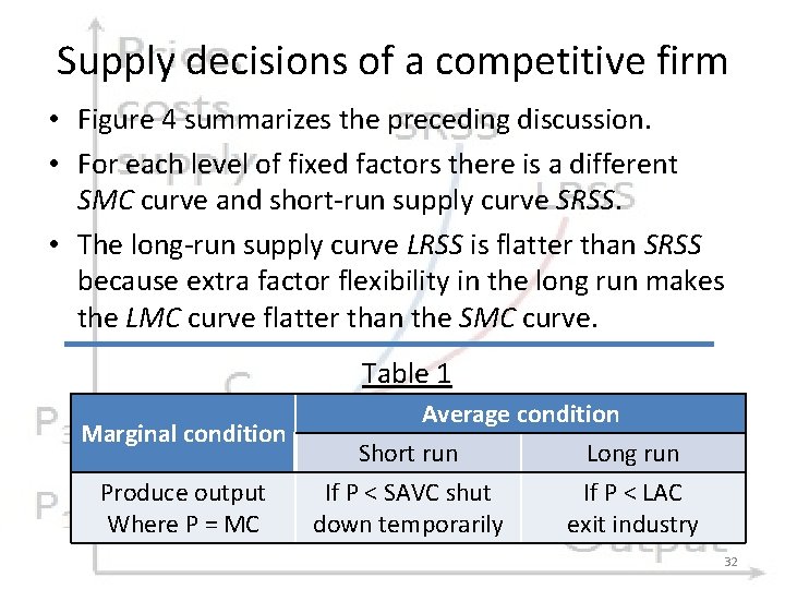
Supply decisions of a competitive firm • Figure 4 summarizes the preceding discussion. • For each level of fixed factors there is a different SMC curve and short-run supply curve SRSS. • The long-run supply curve LRSS is flatter than SRSS because extra factor flexibility in the long run makes the LMC curve flatter than the SMC curve. Table 1 Marginal condition Produce output Where P = MC Average condition Short run Long run If P < SAVC shut If P < LAC down temporarily exit industry 32

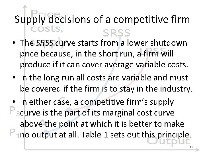
Supply decisions of a competitive firm • The SRSS curve starts from a lower shutdown price because, in the short run, a firm will produce if it can cover average variable costs. • In the long run all costs are variable and must be covered if the firm is to stay in the industry. • In either case, a competitive firm’s supply curve is the part of its marginal cost curve above the point at which it is better to make no output at all. Table 1 sets out this principle. 33

Perfect competition – Industry supply curves Part 2

Industry supply curves • A competitive industry comprises many firms. In the short run two things are fixed: the quantity of fixed factors used by each firm, and the number of firms in the industry. • In the long run, each firm can vary all its factors of production, but the number of firms can also change through entry and exit from the industry. 35

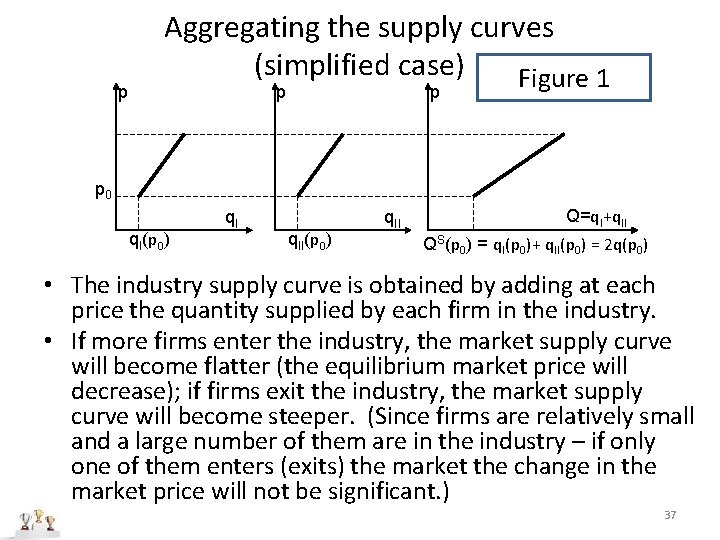
If all firms were identical… • If all firms had the same cost function (the same (perfect) information about the available technologies, equally advantageous locations etc. ) the total quantity supplied would be the quantity supplied by one firm multiplied by the number of firms. • Since the demand curve facing the firm is also the same (horizontal at the market price), the individual supply curves would be identical. 36

p Aggregating the supply curves (simplified case) Figure 1 p p p 0 q. I(p 0) q. II(p 0) q. II Q=q. I+q. II QS(p 0) = q. I(p 0)+ q. II(p 0) = 2 q(p 0) • The industry supply curve is obtained by adding at each price the quantity supplied by each firm in the industry. • If more firms enter the industry, the market supply curve will become flatter (the equilibrium market price will decrease); if firms exit the industry, the market supply curve will become steeper. (Since firms are relatively small and a large number of them are in the industry – if only one of them enters (exits) the market the change in the market price will not be significant. ) 37

Perfect competition in the long run (simplified case) • If there are no barriers to entry, each firm will realize zero economic profit in the long run. (All firms would be at their break-even points: LAC(q*)=LMC(q*)=P*. ) • The number of firms in the industry: n=Q/q, where Q is the equilibrium quantity (Q* = QS(p*)= QD(p*)). • If the firms in the industry realized positive economic profits, other firms would enter the market, driving the market price down. • If the firms in the industry realized negative economic profits, some firms would exit and the market price would rise making the remaining firms more profitable. 38

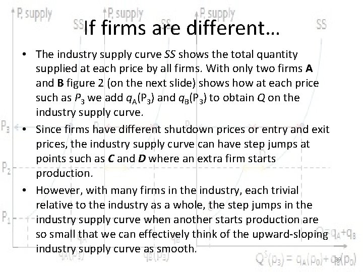
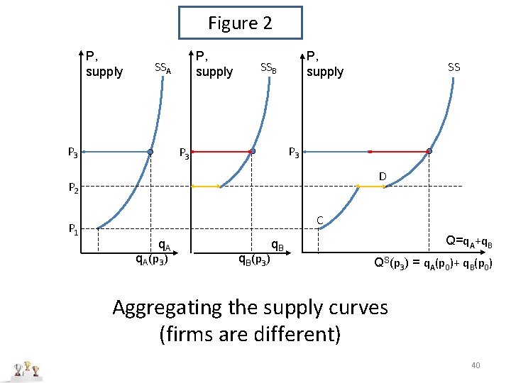
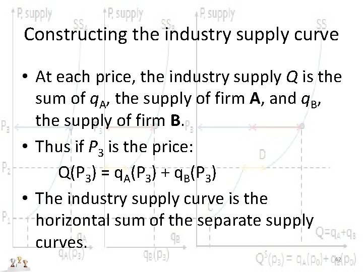
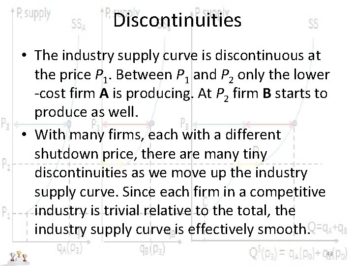
If firms are different… • The industry supply curve SS shows the total quantity supplied at each price by all firms. With only two firms A and B figure 2 (on the next slide) shows how at each price such as P 3 we add q. A(P 3) and q. B(P 3) to obtain Q on the industry supply curve. • Since firms have different shutdown prices or entry and exit prices, the industry supply curve can have step jumps at points such as C and D where an extra firm starts production. • However, with many firms in the industry, each trivial relative to the industry as a whole, the step jumps in the industry supply curve when another starts production are so small that we can effectively think of the upward-sloping industry supply curve as smooth. 39

Figure 2 P, supply SSA P 3 P, supply SSB P 3 D P 2 P 1 SS C q. A(p 3) q. B(p 3) Q=q. A+q. B QS(p 3) = q. A(p 0)+ q. B(p 0) Aggregating the supply curves (firms are different) 40

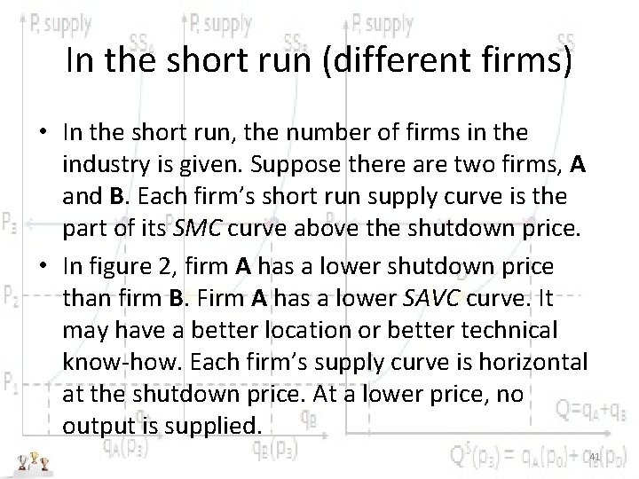
In the short run (different firms) • In the short run, the number of firms in the industry is given. Suppose there are two firms, A and B. Each firm’s short run supply curve is the part of its SMC curve above the shutdown price. • In figure 2, firm A has a lower shutdown price than firm B. Firm A has a lower SAVC curve. It may have a better location or better technical know-how. Each firm’s supply curve is horizontal at the shutdown price. At a lower price, no output is supplied. 41

Constructing the industry supply curve • At each price, the industry supply Q is the sum of q. A, the supply of firm A, and q. B, the supply of firm B. • Thus if P 3 is the price: Q(P 3) = q. A(P 3) + q. B(P 3) • The industry supply curve is the horizontal sum of the separate supply curves. 42

Discontinuities • The industry supply curve is discontinuous at the price P 1. Between P 1 and P 2 only the lower -cost firm A is producing. At P 2 firm B starts to produce as well. • With many firms, each with a different shutdown price, there are many tiny discontinuities as we move up the industry supply curve. Since each firm in a competitive industry is trivial relative to the total, the industry supply curve is effectively smooth. 43

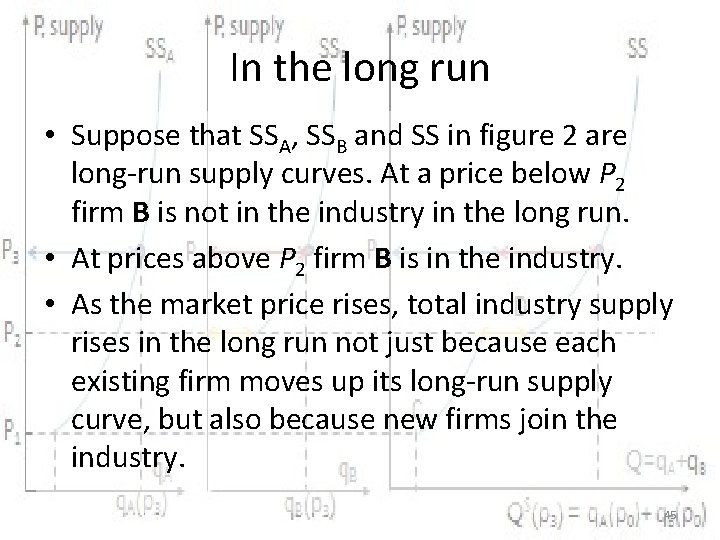
The long-run industry supply curve • Figure 2 may also be used to derive the long-run industry supply curve. For each firm the individual supply curve is the part of its LMC curve above its entry and exit price. • Unlike the short run, the number of firms in the industry is no longer fixed. Existing firms can leave the industry, and new firms can enter. • Instead of horizontally aggregating at each price the quantities supplied by the existing firms in the industry, we must horizontally aggregate the quantities supplied by existing firms and firms that might potentially enter the industry. 44

In the long run • Suppose that SSA, SSB and SS in figure 2 are long-run supply curves. At a price below P 2 firm B is not in the industry in the long run. • At prices above P 2 firm B is in the industry. • As the market price rises, total industry supply rises in the long run not just because each existing firm moves up its long-run supply curve, but also because new firms join the industry. 45

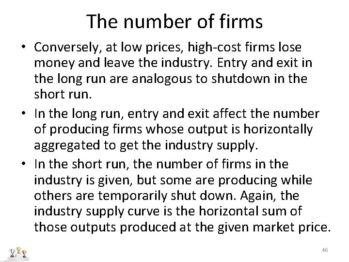
The number of firms • Conversely, at low prices, high-cost firms lose money and leave the industry. Entry and exit in the long run are analogous to shutdown in the short run. • In the long run, entry and exit affect the number of producing firms whose output is horizontally aggregated to get the industry supply. • In the short run, the number of firms in the industry is given, but some are producing while others are temporarily shut down. Again, the industry supply curve is the horizontal sum of those outputs produced at the given market price. 46

Long run and short run compared • The long-run supply curve is flatter than its short-run counterpart. Each firm can vary its factors more appropriately in the long run and has a flatter supply curve. • Moreover, higher prices attract extra firms into the industry. Industry output rises by more than the extra output supplied by the firms already in the industry. 47

• Conversely, if the price falls, firms initially move down their (relatively steep) short-run supply curves. If short-run average variable costs are covered, firms may not reduce output very much. • In the long run each firm reduces output further since all factors of production can now be varied. In addition some firms exit the industry since they are no longer covering long -run average costs. • A price cut reduces industry output by more in the long run than in the short run. 48

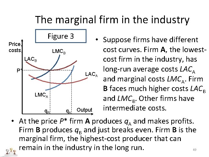
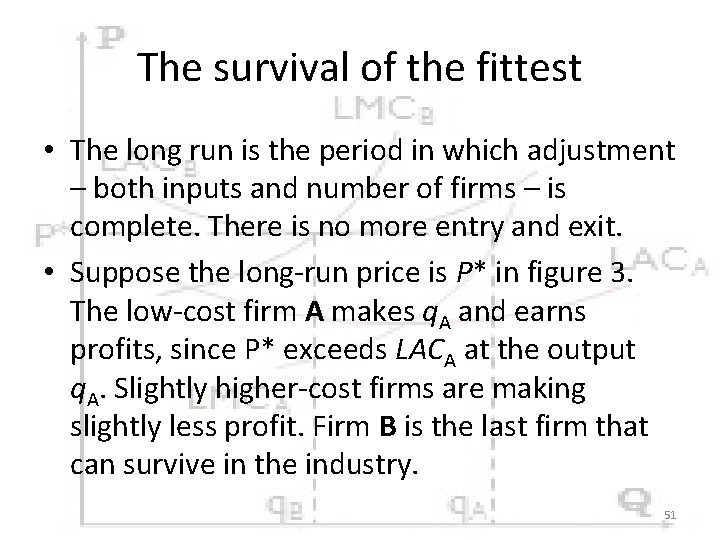
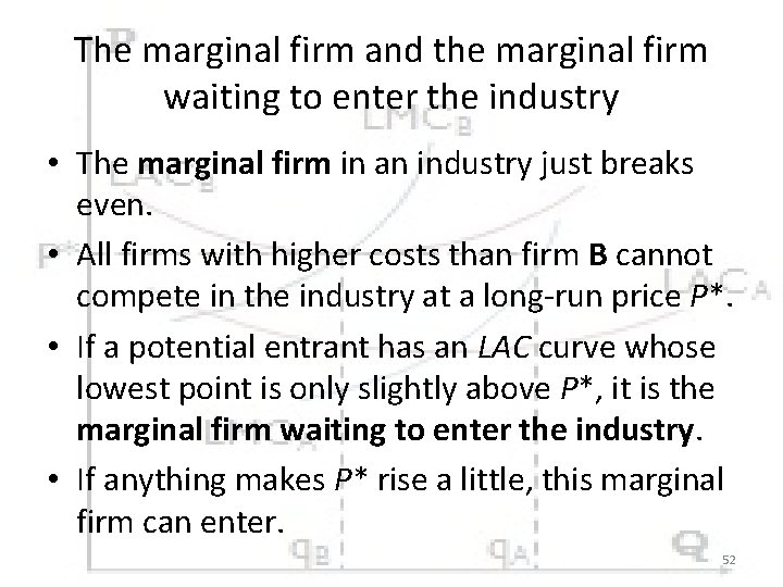
The marginal firm in the industry Figure 3 Price, costs, LMCB LACB P* LMCA q. B q. A • Suppose firms have different cost curves. Firm A, the lowestcost firm in the industry, has long-run average costs LACA and marginal costs LMCA. Firm B faces much higher costs LACB and LMCB. Other firms have intermediate costs. Output • At the price P* firm A produces q. A and makes profits. Firm B produces q. B and just breaks even. Firm B is the marginal firm, the highest-cost producer that can remain in the industry in the long run. 49

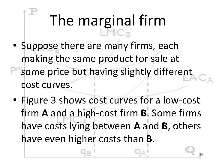
The marginal firm • Suppose there are many firms, each making the same product for sale at some price but having slightly different cost curves. • Figure 3 shows cost curves for a low-cost firm A and a high-cost firm B. Some firms have costs lying between A and B, others have even higher costs than B. 50

The survival of the fittest • The long run is the period in which adjustment – both inputs and number of firms – is complete. There is no more entry and exit. • Suppose the long-run price is P* in figure 3. The low-cost firm A makes q. A and earns profits, since P* exceeds LACA at the output q. A. Slightly higher-cost firms are making slightly less profit. Firm B is the last firm that can survive in the industry. 51

The marginal firm and the marginal firm waiting to enter the industry • The marginal firm in an industry just breaks even. • All firms with higher costs than firm B cannot compete in the industry at a long-run price P*. • If a potential entrant has an LAC curve whose lowest point is only slightly above P*, it is the marginal firm waiting to enter the industry. • If anything makes P* rise a little, this marginal firm can enter. 52

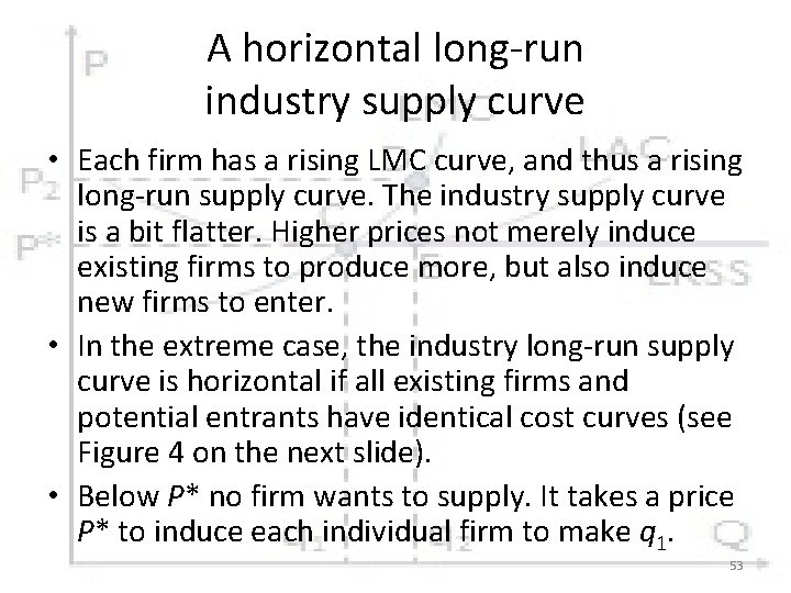
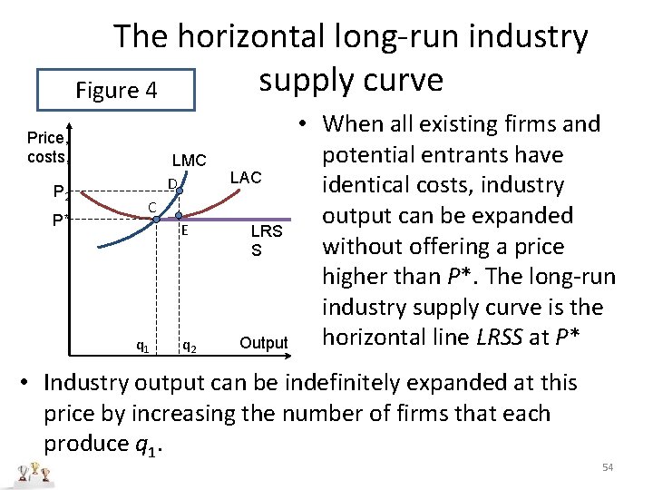
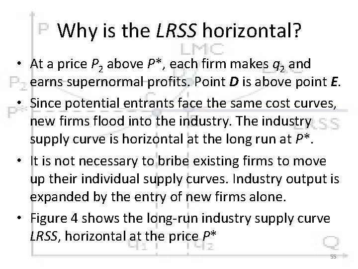
A horizontal long-run industry supply curve • Each firm has a rising LMC curve, and thus a rising long-run supply curve. The industry supply curve is a bit flatter. Higher prices not merely induce existing firms to produce more, but also induce new firms to enter. • In the extreme case, the industry long-run supply curve is horizontal if all existing firms and potential entrants have identical cost curves (see Figure 4 on the next slide). • Below P* no firm wants to supply. It takes a price P* to induce each individual firm to make q 1. 53

The horizontal long-run industry supply curve Figure 4 Price, costs, P 2 P* LMC D LAC C E q 1 q 2 LRS S Output • When all existing firms and potential entrants have identical costs, industry output can be expanded without offering a price higher than P*. The long-run industry supply curve is the horizontal line LRSS at P* • Industry output can be indefinitely expanded at this price by increasing the number of firms that each produce q 1. 54

Why is the LRSS horizontal? • At a price P 2 above P*, each firm makes q 2 and earns supernormal profits. Point D is above point E. • Since potential entrants face the same cost curves, new firms flood into the industry. The industry supply curve is horizontal at the long run at P*. • It is not necessary to bribe existing firms to move up their individual supply curves. Industry output is expanded by the entry of new firms alone. • Figure 4 shows the long-run industry supply curve LRSS, horizontal at the price P* 55

Rising long-run industry supply curves • There are two reasons why a rising longrun industry supply curve is much more likely than a horizontal long-run supply curve for a competitive industry. • First, it is unlikely that every firm and potential firm in the industry has identical cost curves. 56

• Second, even if all firms face the same cost curves, we draw a cost curve for given technology and given input prices. • Although each small firm affects neither output prices nor input prices, collective expansion of output by all firms may bid up input prices. • It then needs a higher output price to induce industry output to rise. In general, the longrun industry supply curve slopes up. 57

Pure monopoly Part 3

A perfectly competitive firm and a monopolist • A perfectly competitive firm is too small to worry about any effect of its output decision on industry supply and hence price. It can sell as much as it wants at the market price. • A monopolist is the sole supplier and potential supplier of the industry’s product. A real monopolist need not worry about entry even in the long run. 59

A monopolist and the industry • The firm and the industry coincide. The sole national supplier may not be a monopolist if the good or service is internationally traded. • Royal Mail (formerly Consignia) is the sole supplier of UK stamps and a monopolist in them. Airbus is the only large plane-maker in Europe, but is not a monopolist since it faces cutthroat international competition from Boeing. Sole suppliers may also face invisible competition from potential entrants. If so, they are not monopolists. 60

Profit maximizing output • To maximize profits any firm chooses the output at which marginal revenue MR equals marginal cost (SMC in the short run LMC in the long run). • It then checks whether it is covering average costs (SAVC in the short run and LAC in the long run). 61

A competitive firm’s supply decision • The special feature of a competitive firm is that MR equals price. • Selling an extra unit of output does not bid down the price and reduce the revenue earned on previous units. The price at which the extra unit is sold is the change in total revenue. 62

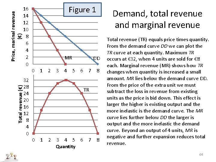
The monopolist’s demand curve • In contrast, the monopolist’s demand curve is the industry demand curve, which slopes down. • Hence, MR is less than the price at which the extra output is sold. • The monopolist knows that extra output reduces revenue from existing units. To sell more, the price on all units must be cut. 63

Total revenue (€) Price, marinal revenue (€) 16 14 12 10 8 6 4 2 0 32 28 24 20 16 12 8 4 0 Figure 1 MR DD 0 1 2 3 4 5 6 7 8 TR 0 1 2 3 4 5 6 7 8 Quantity Demand, total revenue and marginal revenue Total revenue (TR) equals price times quantity. From the demand curve DD we can plot the TR curve at each quantity. Maximum TR occurs at € 32, when 4 units are sold for € 8 each. Marginal revenue (MR) shows how TR changes when quantity is increased a small amount. MR lies below the demand curve DD. From the price of the extra unit we must subtract the loss in revenue from existing units as the price is bid down. This effect is larger the higher is existing output and the more inelastic is the demand curve. The MR curve lies further below DD the larger is output and the more inelastic the demand curve. Beyond an output of 4 units, MR is negative and further expansion reduces total revenue. 64

Price, MR and TR • The more inelastic the demand curve, the more an extra unit of output bids down the price, reducing revenue from existing units. • At any output, MR is further below the demand curve the more inelastic is demand. • Also, the larger the existing output, the larger the revenue loss from existing units when the price is reduced to sell another unit. • For a given demand curve, MR falls increasingly below price the higher the output from which we begin. 65

Revenue and cost • Beyond a certain output (4 in figure 1), the revenue loss on existing output exceeds the revenue gain from the extra unit itself. Marginal revenue is negative. Further expansion reduces total revenue. • On the cost side, with only one product, the cost curves of a single firm carry over directly. The monopolist has the usual cost curves, average and marginal, short-run and long-run. • For simplicity, we discuss only the long-run curves in detail. 66

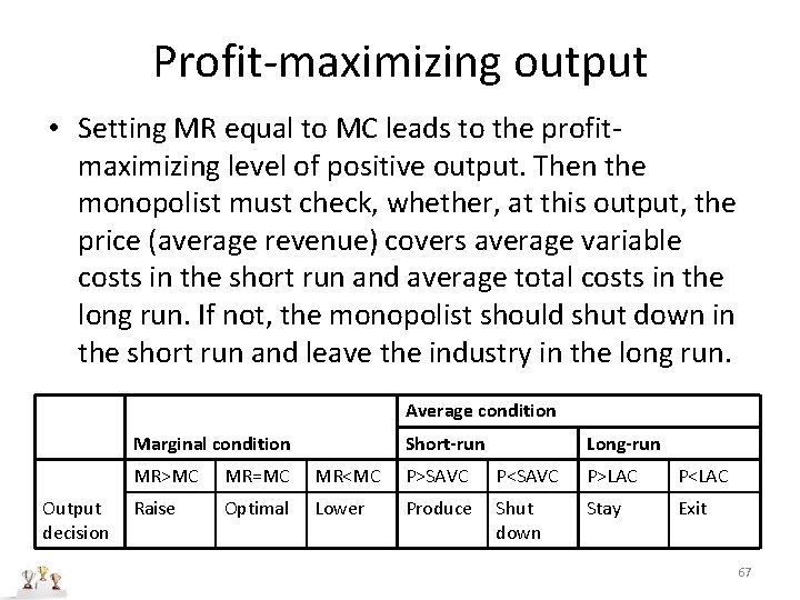
Profit-maximizing output • Setting MR equal to MC leads to the profitmaximizing level of positive output. Then the monopolist must check, whether, at this output, the price (average revenue) covers average variable costs in the short run and average total costs in the long run. If not, the monopolist should shut down in the short run and leave the industry in the long run. Average condition Short-run Marginal condition Output decision Long-run MR>MC MR=MC MR<MC P>SAVC P<SAVC P>LAC P<LAC Raise Optimal Lower Produce Shut down Stay Exit 67

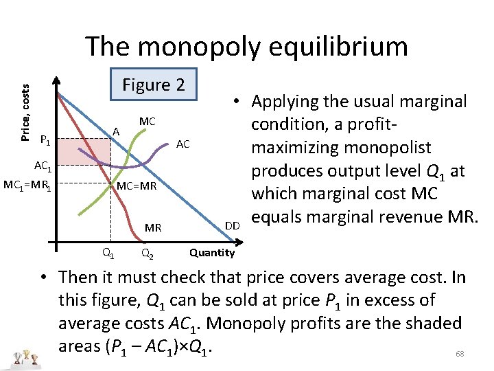
Price, costs The monopoly equilibrium Figure 2 P 1 A MC AC AC 1 MC 1=MR 1 MC=MR MR Q 1 Q 2 • Applying the usual marginal condition, a profitmaximizing monopolist produces output level Q 1 at which marginal cost MC equals marginal revenue MR. DD Quantity • Then it must check that price covers average cost. In this figure, Q 1 can be sold at price P 1 in excess of average costs AC 1. Monopoly profits are the shaded areas (P 1 – AC 1)×Q 1. 68

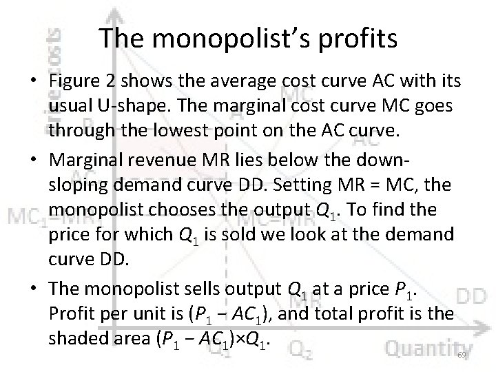
The monopolist’s profits • Figure 2 shows the average cost curve AC with its usual U-shape. The marginal cost curve MC goes through the lowest point on the AC curve. • Marginal revenue MR lies below the downsloping demand curve DD. Setting MR = MC, the monopolist chooses the output Q 1. To find the price for which Q 1 is sold we look at the demand curve DD. • The monopolist sells output Q 1 at a price P 1. Profit per unit is (P 1 − AC 1), and total profit is the shaded area (P 1 − AC 1)×Q 1. 69

Supernormal (monopoly) profits • Even in the long run, the monopolist makes supernormal profits, sometimes called monopoly profits. • Unlike the competitive industry, supernormal profits of a monopolist are not eliminated by entry of more firms and a fall in the price. • A monopoly has no fear of possible entry. By ruling out entry, we remove the mechanism by which supernormal profits disappear in the long run. 70

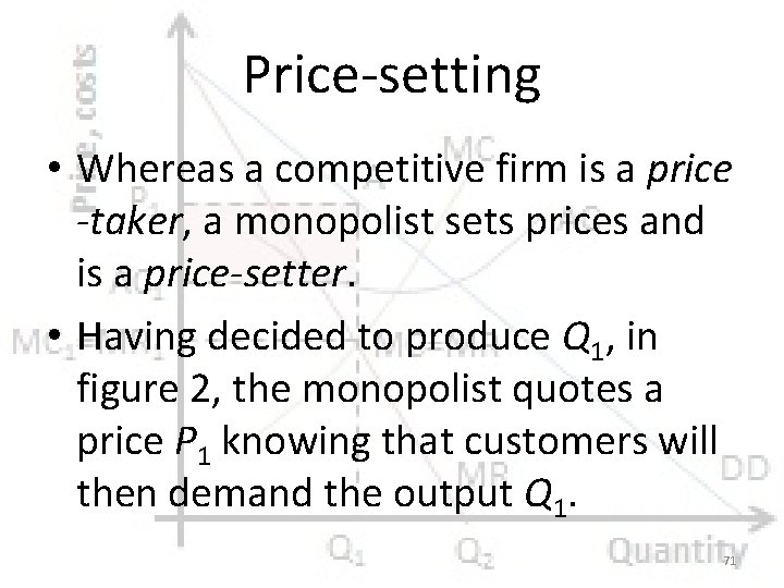
Price-setting • Whereas a competitive firm is a price -taker, a monopolist sets prices and is a price-setter. • Having decided to produce Q 1, in figure 2, the monopolist quotes a price P 1 knowing that customers will then demand the output Q 1. 71

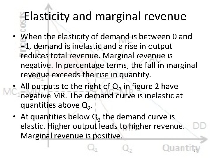
Elasticity and marginal revenue • When the elasticity of demand is between 0 and − 1, demand is inelastic and a rise in output reduces total revenue. Marginal revenue is negative. In percentage terms, the fall in marginal revenue exceeds the rise in quantity. • All outputs to the right of Q 2 in figure 2 have negative MR. The demand curve is inelastic at quantities above Q 2. • At quantities below Q 2 the demand curve is elastic. Higher output leads to higher revenue. Marginal revenue is positive. 72

A monopolist never produces on the inelastic part of the demand curve • • The monopolist sets MC = MR. Since MC must be positive, so must MR. The chosen output must lie to the left of Q 2. A monopolist never produces on the inelastic part of the demand curve. 73

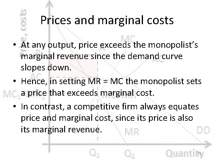
Prices and marginal costs • At any output, price exceeds the monopolist’s marginal revenue since the demand curve slopes down. • Hence, in setting MR = MC the monopolist sets a price that exceeds marginal cost. • In contrast, a competitive firm always equates price and marginal cost, since its price is also its marginal revenue. 74

Monopoly power • The excess of price over marginal cost is a measure of monopoly power. • A competitive firm cannot raise the price above marginal cost and has no monopoly power. The more inelastic the demand curve of the monopolist, the more marginal revenue is below price, the greater is the excess of price over marginal cost, and the more monopoly power it has. 75

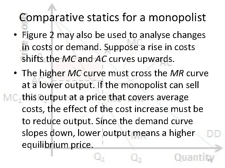
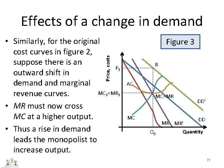
Comparative statics for a monopolist • Figure 2 may also be used to analyse changes in costs or demand. Suppose a rise in costs shifts the MC and AC curves upwards. • The higher MC curve must cross the MR curve at a lower output. If the monopolist can sell this output at a price that covers average costs, the effect of the cost increase must be to reduce output. Since the demand curve slopes down, lower output means a higher equilibrium price. 76

Effects of a change in demand Price, costs • Similarly, for the original cost curves in figure 2, suppose there is an P 3 outward shift in demand marginal MC 3=MR 3 revenue curves. • MR must now cross MC at a higher output. • Thus a rise in demand leads the monopolist to increase output. Figure 3 B AC MC=MR MC DD’ MR MR’ Q 3 DD Quantity 77

Comparing a perfectly competitive industry with a monopoly • We now compare a perfectly competitive industry with a monopoly. • For this comparison to be of interest the two industries must face the same demand cost conditions. How would the same industry change if it were organized first as a competitive industry then as a monopoly? • Can the same industry be both competitive and a monopoly? Only in some special cases. 78

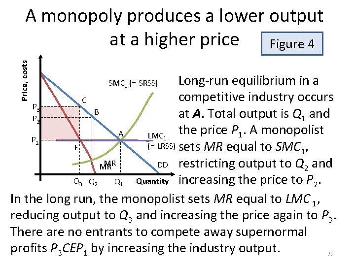
Price, costs A monopoly produces a lower output at a higher price Figure 4 Long-run equilibrium in a competitive industry occurs C P 3 B at A. Total output is Q 1 and P 2 the price P 1. A monopolist A LMC 1 P 1 (= LRSS) sets MR equal to SMC , E 1 MR DD restricting output to Q 2 and MR Q 3 Q 2 Q 1 Quantity increasing the price to P 2. In the long run, the monopolist sets MR equal to LMC 1, reducing output to Q 3 and increasing the price again to P 3. There are no entrants to compete away supernormal profits P 3 CEP 1 by increasing the industry output. 79 SMC 1 (= SRSS)

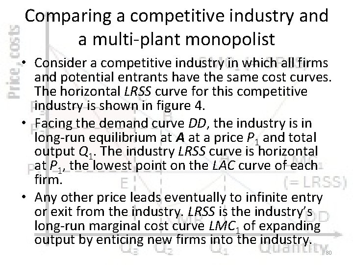
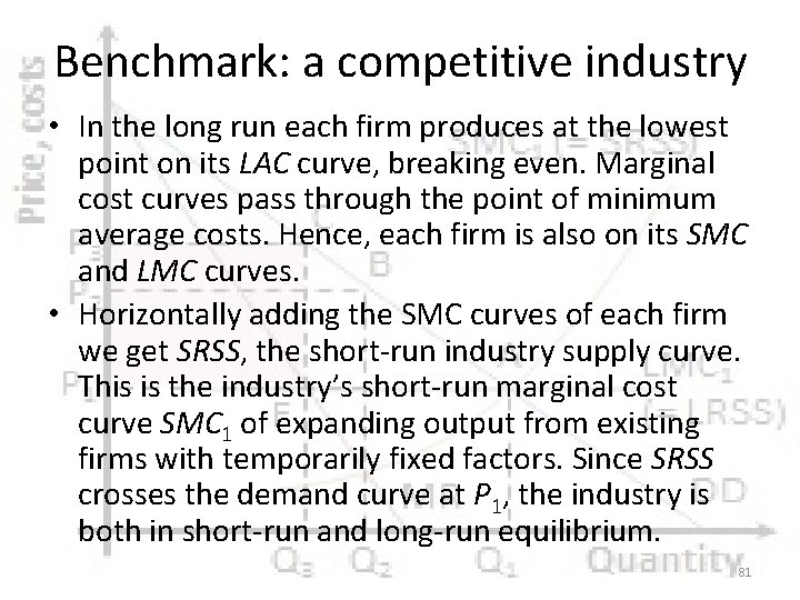
Comparing a competitive industry and a multi-plant monopolist • Consider a competitive industry in which all firms and potential entrants have the same cost curves. The horizontal LRSS curve for this competitive industry is shown in figure 4. • Facing the demand curve DD, the industry is in long-run equilibrium at A at a price P 1 and total output Q 1. The industry LRSS curve is horizontal at P 1, the lowest point on the LAC curve of each firm. • Any other price leads eventually to infinite entry or exit from the industry. LRSS is the industry’s long-run marginal cost curve LMC 1 of expanding output by enticing new firms into the industry. 80

Benchmark: a competitive industry • In the long run each firm produces at the lowest point on its LAC curve, breaking even. Marginal cost curves pass through the point of minimum average costs. Hence, each firm is also on its SMC and LMC curves. • Horizontally adding the SMC curves of each firm we get SRSS, the short-run industry supply curve. This is the industry’s short-run marginal cost curve SMC 1 of expanding output from existing firms with temporarily fixed factors. Since SRSS crosses the demand curve at P 1, the industry is both in short-run and long-run equilibrium. 81

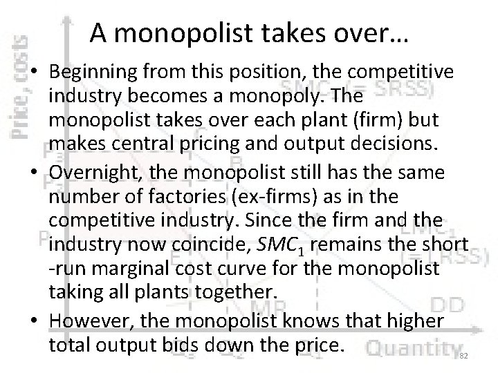
A monopolist takes over… • Beginning from this position, the competitive industry becomes a monopoly. The monopolist takes over each plant (firm) but makes central pricing and output decisions. • Overnight, the monopolist still has the same number of factories (ex-firms) as in the competitive industry. Since the firm and the industry now coincide, SMC 1 remains the short -run marginal cost curve for the monopolist taking all plants together. • However, the monopolist knows that higher total output bids down the price. 82

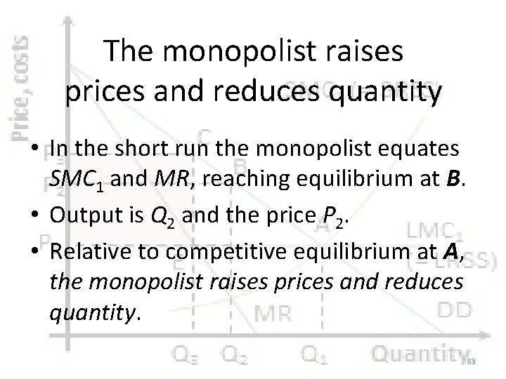
The monopolist raises prices and reduces quantity • In the short run the monopolist equates SMC 1 and MR, reaching equilibrium at B. • Output is Q 2 and the price P 2. • Relative to competitive equilibrium at A, the monopolist raises prices and reduces quantity. 83

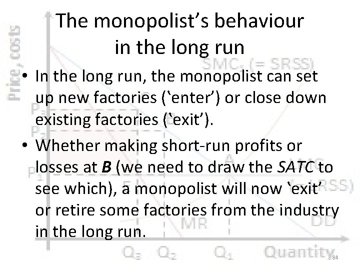
The monopolist’s behaviour in the long run • In the long run, the monopolist can set up new factories (‛enter’) or close down existing factories (‛exit’). • Whether making short-run profits or losses at B (we need to draw the SATC to see which), a monopolist will now ‛exit’ or retire some factories from the industry in the long run. 84

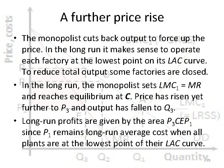
A further price rise • The monopolist cuts back output to force up the price. In the long run it makes sense to operate each factory at the lowest point on its LAC curve. To reduce total output some factories are closed. • In the long run, the monopolist sets LMC 1 = MR and reaches equilibrium at C. Price has risen yet further to P 3 and output has fallen to Q 3. • Long-run profits are given by the area P 3 CEP 1 since P 1 remains long-run average cost when all plants are at the lowest point of their LAC curve. 85

Absence of entry • Because MR is less than price, a monopolist produces less than a competitive industry and charges a higher price. • However, in this example it is a legal prohibition on entry by competitors that allows the monopolist to succeed in the long run. Otherwise, with identical cost curves, other firms would set up in competition, expand industry output, and compete away these supernormal profits. Absence of entry is intrinsic to the model of monopoly. 86

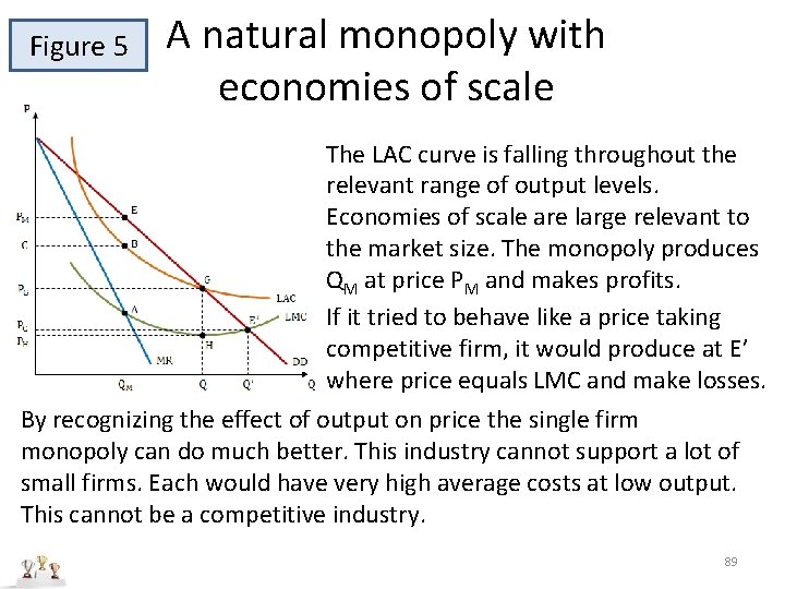
A single-plant monopolist • Instead of a multi-plant monopolist taking over many previously competitive firms, consider a monopolist meeting the entire industry demand from a single plant. • This is most plausible when scale economies are big. There are huge costs in setting up a national telephone network. Yet the cost of connecting a marginal subscriber is low once the network has been set up. 87

Natural monopolies • Monopolies enjoying huge economies of scale – falling LAC curves over the entire range of output – are natural monopolies. • Large-scale economies may explain why there is a sole supplier without fear of entry by others. • Smaller entrants would be at a prohibitive cost disadvantage. 88

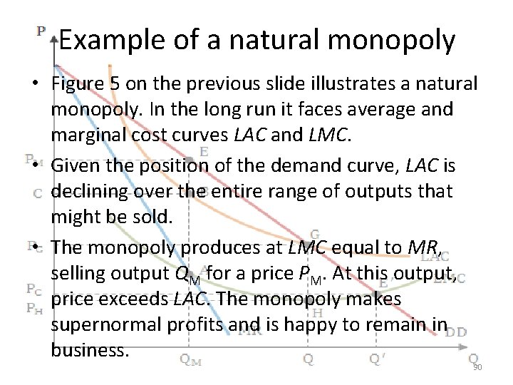
Figure 5 A natural monopoly with economies of scale The LAC curve is falling throughout the relevant range of output levels. Economies of scale are large relevant to the market size. The monopoly produces QM at price PM and makes profits. If it tried to behave like a price taking competitive firm, it would produce at E’ where price equals LMC and make losses. By recognizing the effect of output on price the single firm monopoly can do much better. This industry cannot support a lot of small firms. Each would have very high average costs at low output. This cannot be a competitive industry. 89

Example of a natural monopoly • Figure 5 on the previous slide illustrates a natural monopoly. In the long run it faces average and marginal cost curves LAC and LMC. • Given the position of the demand curve, LAC is declining over the entire range of outputs that might be sold. • The monopoly produces at LMC equal to MR, selling output QM for a price PM. At this output, price exceeds LAC. The monopoly makes supernormal profits and is happy to remain in business. 90

• It makes no sense to compare this equilibrium with how the industry would behave if it were competitive. With such economies of scale there is only one firm in the industry. • LAC is the cost curve for each possible firm. If a lot of small firms each produced a small fraction of total output, their average costs would be huge. By expanding, a single firm could undercut them and wipe them out. • This industry must have a sole supplier. This natural monopoly will maximize profits only by recognizing that its marginal revenue is not its price. 91

A discriminating monopolist • A discriminating monopolist charges different prices to different customers. • To equate the marginal revenue from different groups, groups with an inelastic demand must pay a higher price. • Successful price discrimination requires that customers cannot trade the product among themselves. 92

Monopoly and technical change • Monopolies may have more internal resources available for research and may have a higher incentive for cost-saving research because the profits from technical advances will not be eroded by entry. • Although small firms do not undertake much expensive research, it appears that the patent laws provide adequate incentives for mediumand larger-sized firms. There is no evidence that an industry has to be a monopoly to undertake cost-saving research. 93