UNDERSTANDING STATISTIC EXPERIMENTAL DESIGN Understanding Statistics Experimental Design

UNDERSTANDING STATISTIC & EXPERIMENTAL DESIGN Understanding Statistics & Experimental Design 1

Content 1. Basic Probability Theory 2. Signal Detection Theory (SDT) 3. SDT and Statistics I and II 4. Statistics in a nutshell 5. Multiple Testing 6. ANOVA 7. Experimental Design & Statistics 8. Correlations & PCA 9. Meta-Statistics: Basics 10. Meta-Statistics: Too good to be true 11. Meta-Statistics: How big a problem is publication bias? 12. Meta-Statistics: What do we do now? Understanding Statistics & Experimental Design 2

Effect sizes, power, and violations of hypothesis testing Understanding Statistics & Experimental Design 3

Experiments We run experiments to test specific hypotheses about population parameters H 0: μ 1=μ 2 H 0: μ=3 We gather data from samples to try to infer something about the populations The fundamental question in hypothesis testing is whether the population effect is big enough to not be attributed to chance from random sampling We want to quantify “big enough” Understanding Statistics & Experimental Design 4

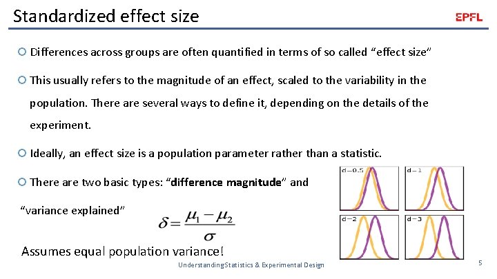
Standardized effect size Differences across groups are often quantified in terms of so called “effect size” This usually refers to the magnitude of an effect, scaled to the variability in the population. There are several ways to define it, depending on the details of the experiment. Ideally, an effect size is a population parameter rather than a statistic. There are two basic types: “difference magnitude” and “variance explained” Assumes equal population variance! Understanding Statistics & Experimental Design 5

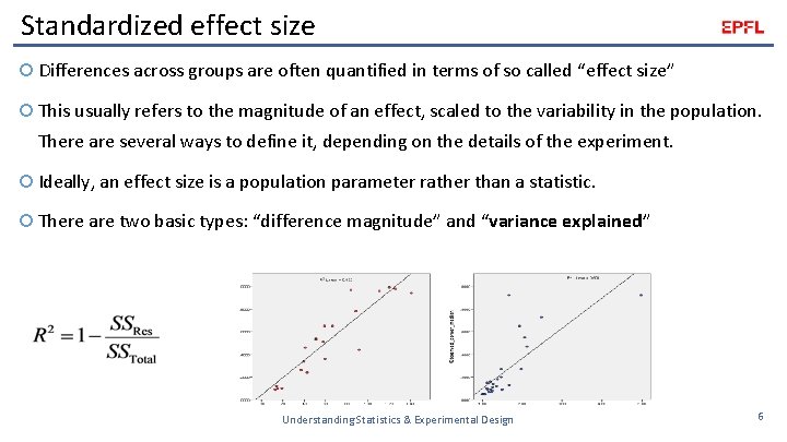
Standardized effect size Differences across groups are often quantified in terms of so called “effect size” This usually refers to the magnitude of an effect, scaled to the variability in the population. There are several ways to define it, depending on the details of the experiment. Ideally, an effect size is a population parameter rather than a statistic. There are two basic types: “difference magnitude” and “variance explained” Understanding Statistics & Experimental Design 6

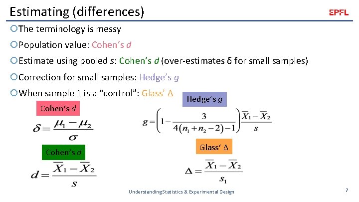
Estimating (differences) The terminology is messy Population value: Cohen’s d Estimate using pooled s: Cohen’s d (over-estimates δ for small samples) Correction for small samples: Hedge’s g When sample 1 is a “control”: Glass’ Δ Cohen’s d Hedge’s g Glass’ Δ Understanding Statistics & Experimental Design 7

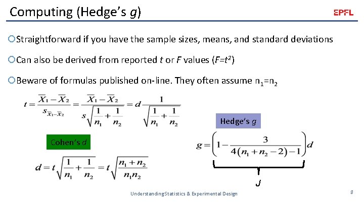
Computing (Hedge’s g) Straightforward if you have the sample sizes, means, and standard deviations Can also be derived from reported t or F values (F=t 2) Beware of formulas published on-line. They often assume n 1=n 2 Hedge’s g Cohen’s d J Understanding Statistics & Experimental Design 8

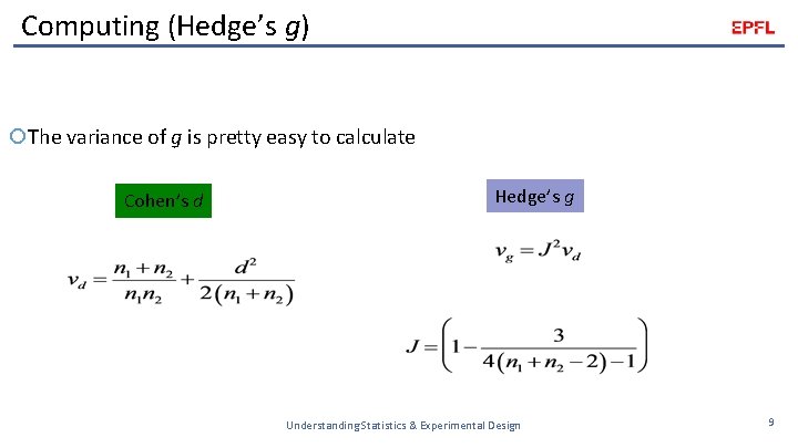
Computing (Hedge’s g) The variance of g is pretty easy to calculate Cohen’s d Hedge’s g Understanding Statistics & Experimental Design 9

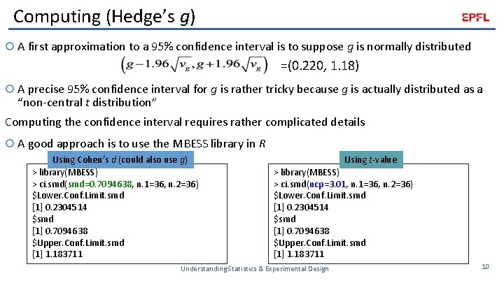
Computing (Hedge’s g) A first approximation to a 95% confidence interval is to suppose g is normally distributed =(0. 220, 1. 18) A precise 95% confidence interval for g is rather tricky because g is actually distributed as a “non-central t distribution” Computing the confidence interval requires rather complicated details A good approach is to use the MBESS library in R Using Cohen’s d (could also use g) > library(MBESS) > ci. smd(smd=0. 7094638, n. 1=36, n. 2=36) $Lower. Conf. Limit. smd [1] 0. 2304514 $smd [1] 0. 7094638 $Upper. Conf. Limit. smd [1] 1. 183711 Using t-value > library(MBESS) > ci. smd(ncp=3. 01, n. 1=36, n. 2=36) $Lower. Conf. Limit. smd [1] 0. 2304514 $smd [1] 0. 7094638 $Upper. Conf. Limit. smd [1] 1. 183711 Understanding Statistics & Experimental Design 10

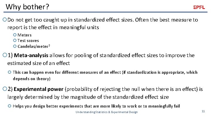
Why bother? Do not get too caught up in standardized effect sizes. Often the best measure to report is the effect in meaningful units Meters Test scores Candelas/meter 2 1) Meta-analysis allows for pooling of standardized effect sizes to improve the estimated size of an effect This can happen even for different measures of an effect (if standardization is appropriate, which depends on theory) 2) Experimental power (probability of rejecting the null when there is an effect) is largely determined by the magnitude of the standardized effect size Helps you design better experiments that are more likely to work or to meaningfully fail Understanding Statistics & Experimental Design 11

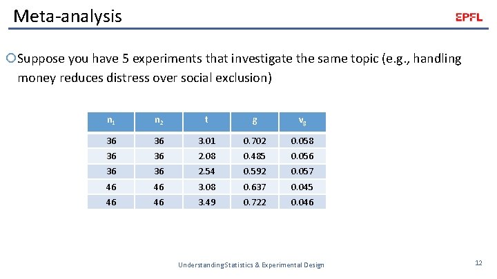
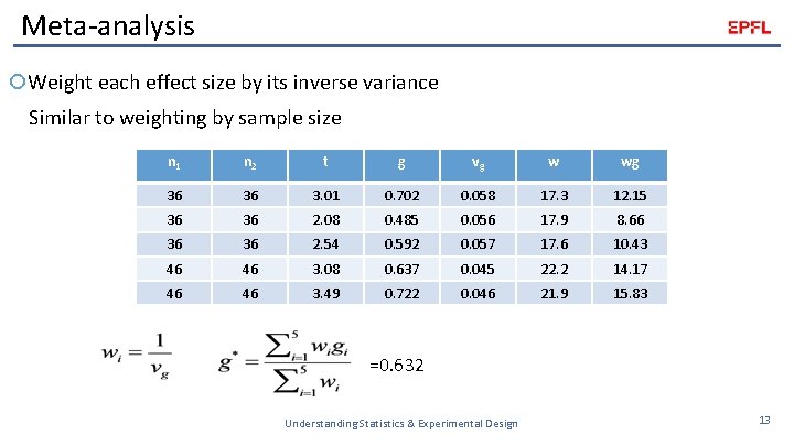
Meta-analysis Suppose you have 5 experiments that investigate the same topic (e. g. , handling money reduces distress over social exclusion) n 1 n 2 t g vg 36 36 3. 01 0. 702 0. 058 36 36 2. 08 0. 485 0. 056 36 36 2. 54 0. 592 0. 057 46 46 3. 08 0. 637 0. 045 46 46 3. 49 0. 722 0. 046 Understanding Statistics & Experimental Design 12

Meta-analysis Weight each effect size by its inverse variance Similar to weighting by sample size n 1 n 2 t g vg w wg 36 36 3. 01 0. 702 0. 058 17. 3 12. 15 36 36 2. 08 0. 485 0. 056 17. 9 8. 66 36 36 2. 54 0. 592 0. 057 17. 6 10. 43 46 46 3. 08 0. 637 0. 045 22. 2 14. 17 46 46 3. 49 0. 722 0. 046 21. 9 15. 83 =0. 632 Understanding Statistics & Experimental Design 13

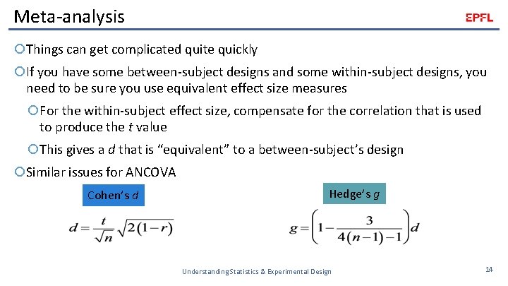
Meta-analysis Things can get complicated quite quickly If you have some between-subject designs and some within-subject designs, you need to be sure you use equivalent effect size measures For the within-subject effect size, compensate for the correlation that is used to produce the t value This gives a d that is “equivalent” to a between-subject’s design Similar issues for ANCOVA Cohen’s d Hedge’s g Understanding Statistics & Experimental Design 14

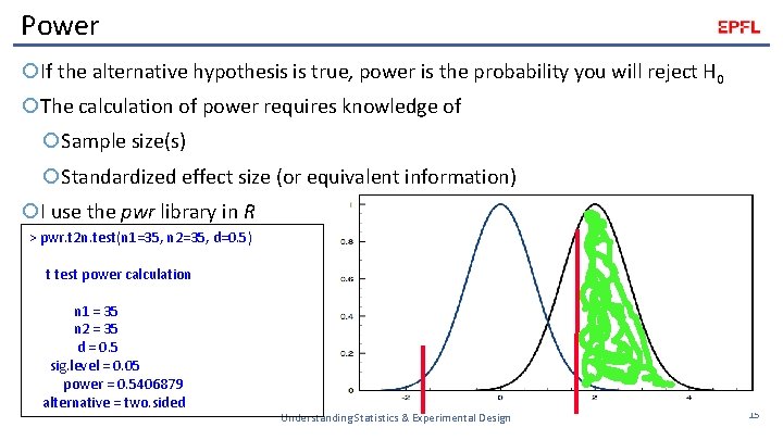
Power If the alternative hypothesis is true, power is the probability you will reject H 0 The calculation of power requires knowledge of Sample size(s) Standardized effect size (or equivalent information) I use the pwr library in R > pwr. t 2 n. test(n 1=35, n 2=35, d=0. 5) t test power calculation n 1 = 35 n 2 = 35 d = 0. 5 sig. level = 0. 05 power = 0. 5406879 alternative = two. sided Understanding Statistics & Experimental Design 15

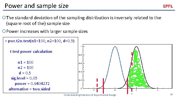
Power and sample size The standard deviation of the sampling distribution is inversely related to the (square root of the) sample size Power increases with larger sample sizes > pwr. t 2 n. test(n 1=100, n 2=100, d=0. 5) t test power calculation n 1 = 100 n 2 = 100 d = 0. 5 sig. level = 0. 05 power = 0. 9404272 alternative = two. sided Understanding Statistics & Experimental Design 16

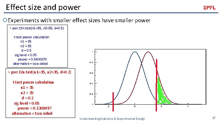
Effect size and power Experiments with smaller effect sizes have smaller power > pwr. t 2 n. test(n 1=35, n 2=35, d=0. 5) t test power calculation n 1 = 35 n 2 = 35 d = 0. 5 sig. level = 0. 05 power = 0. 5406879 alternative = two. sided > pwr. t 2 n. test(n 1=35, n 2=35, d=0. 2) t test power calculation n 1 = 35 n 2 = 35 d = 0. 2 sig. level = 0. 05 power = 0. 1308497 alternative = two. sided Understanding Statistics & Experimental Design 17

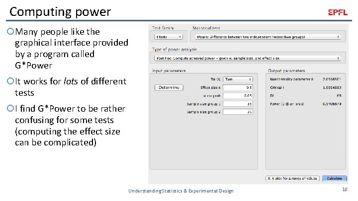
Computing power Many people like the graphical interface provided by a program called G*Power It works for lots of different tests I find G*Power to be rather confusing for some tests (computing the effect size can be complicated) Understanding Statistics & Experimental Design 18

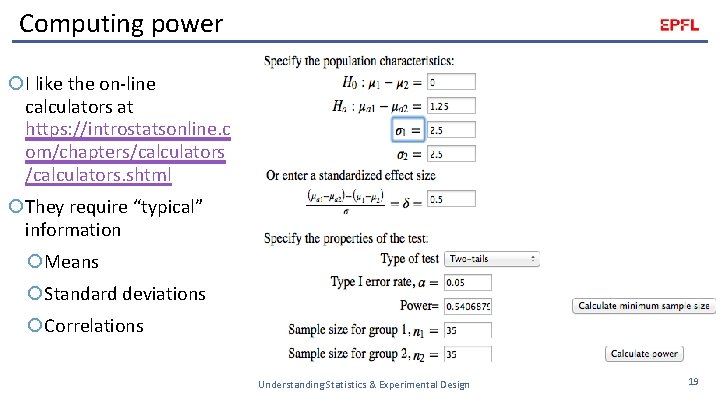
Computing power I like the on-line calculators at https: //introstatsonline. c om/chapters/calculators. shtml They require “typical” information Means Standard deviations Correlations Understanding Statistics & Experimental Design 19

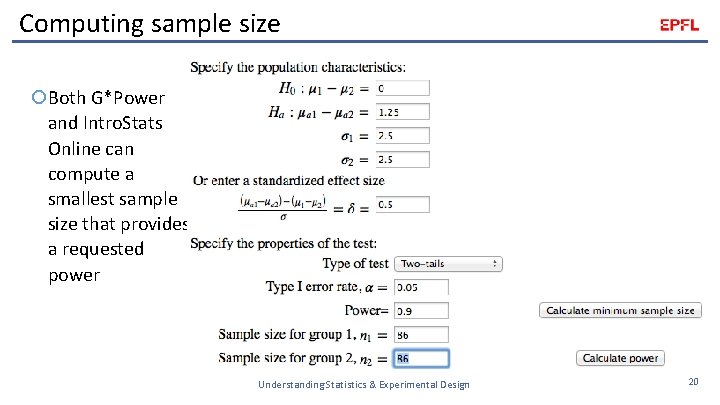
Computing sample size Both G*Power and Intro. Stats Online can compute a smallest sample size that provides a requested power Understanding Statistics & Experimental Design 20

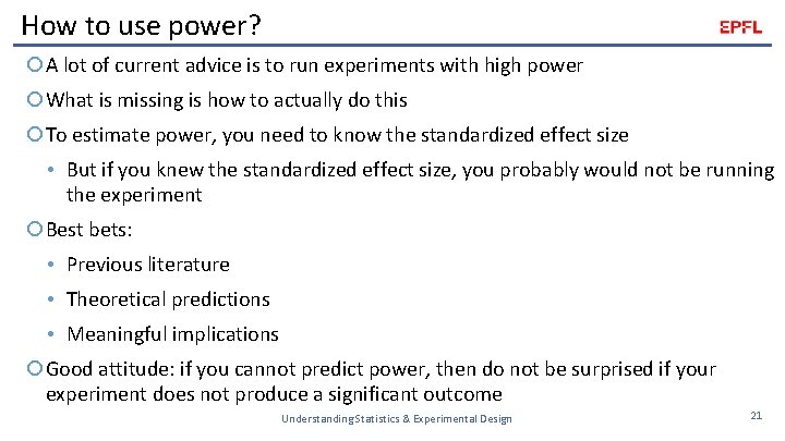
How to use power? A lot of current advice is to run experiments with high power What is missing is how to actually do this To estimate power, you need to know the standardized effect size • But if you knew the standardized effect size, you probably would not be running the experiment Best bets: • Previous literature • Theoretical predictions • Meaningful implications Good attitude: if you cannot predict power, then do not be surprised if your experiment does not produce a significant outcome Understanding Statistics & Experimental Design 21

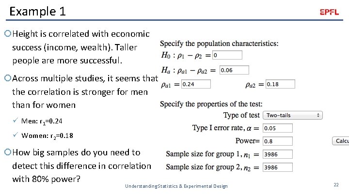
Example 1 Height is correlated with economic success (income, wealth). Taller people are more successful. Across multiple studies, it seems that the correlation is stronger for men than for women ü Men: r 1=0. 24 ü Women: r 2=0. 18 How big samples do you need to detect this difference in correlation with 80% power? Understanding Statistics & Experimental Design 22

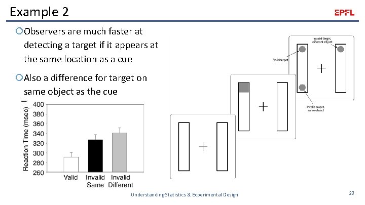
Example 2 Observers are much faster at detecting a target if it appears at the same location as a cue Also a difference for target on same object as the cue Understanding Statistics & Experimental Design 23

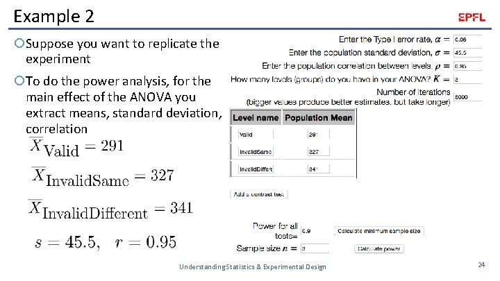
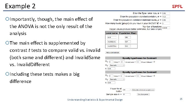
Example 2 Suppose you want to replicate the experiment To do the power analysis, for the main effect of the ANOVA you extract means, standard deviation, correlation Understanding Statistics & Experimental Design 24

Example 2 Importantly, though, the main effect of the ANOVA is not the only result of the analysis The main effect is supplemented by contrast t tests to compare valid vs. invalid (both same and different) and Invalid. Same vs. Invalid. Different Including these tests makes a big difference Understanding Statistics & Experimental Design 25

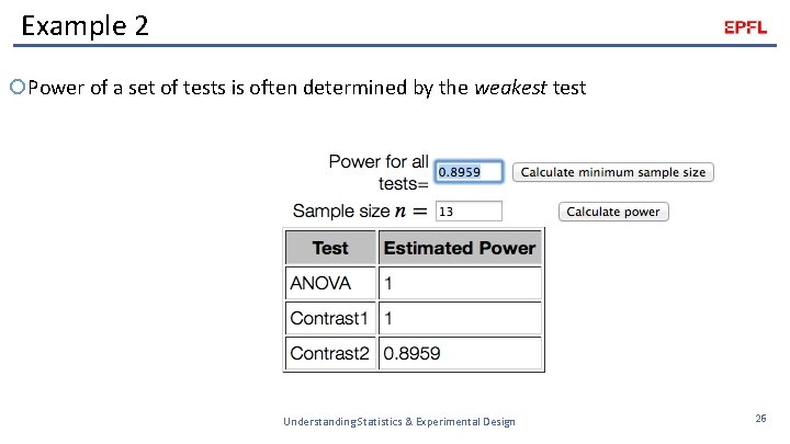
Example 2 Power of a set of tests is often determined by the weakest test Understanding Statistics & Experimental Design 26

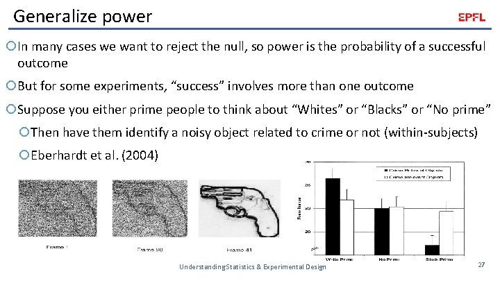
Generalize power In many cases we want to reject the null, so power is the probability of a successful outcome But for some experiments, “success” involves more than one outcome Suppose you either prime people to think about “Whites” or “Blacks” or “No prime” Then have them identify a noisy object related to crime or not (within-subjects) Eberhardt et al. (2004) Understanding Statistics & Experimental Design 27

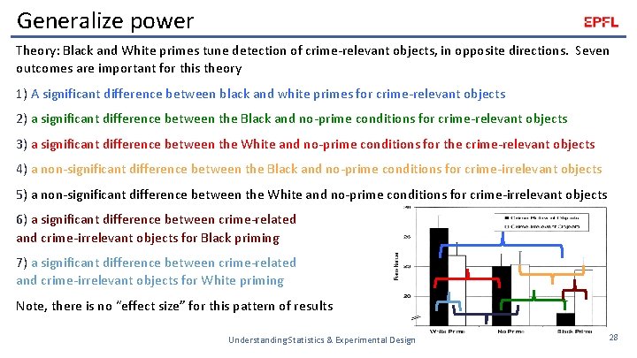
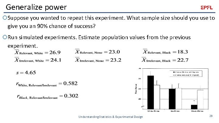
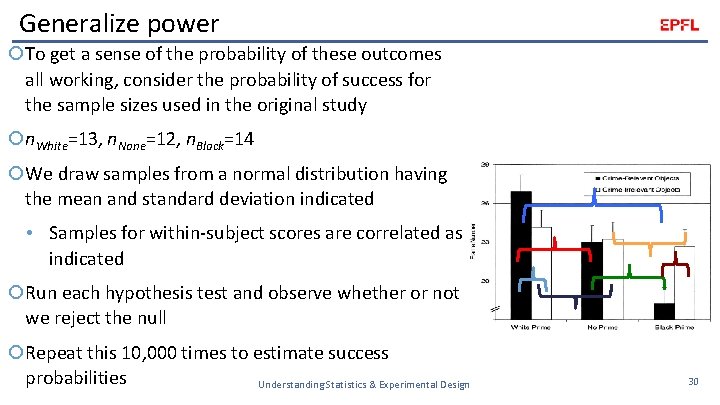
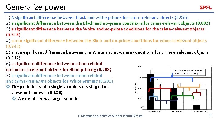
Generalize power Theory: Black and White primes tune detection of crime-relevant objects, in opposite directions. Seven outcomes are important for this theory 1) A significant difference between black and white primes for crime-relevant objects 2) a significant difference between the Black and no-prime conditions for crime-relevant objects 3) a significant difference between the White and no-prime conditions for the crime-relevant objects 4) a non-significant difference between the Black and no-prime conditions for crime-irrelevant objects 5) a non-significant difference between the White and no-prime conditions for crime-irrelevant objects 6) a significant difference between crime-related and crime-irrelevant objects for Black priming 7) a significant difference between crime-related and crime-irrelevant objects for White priming Note, there is no “effect size” for this pattern of results Understanding Statistics & Experimental Design 28

Generalize power Suppose you wanted to repeat this experiment. What sample size should you use to give you an 90% chance of success? Run simulated experiments. Estimate population values from the previous experiment. Understanding Statistics & Experimental Design 29

Generalize power To get a sense of the probability of these outcomes all working, consider the probability of success for the sample sizes used in the original study n. White=13, n. None=12, n. Black=14 We draw samples from a normal distribution having the mean and standard deviation indicated • Samples for within-subject scores are correlated as indicated Run each hypothesis test and observe whether or not we reject the null Repeat this 10, 000 times to estimate success probabilities Understanding Statistics & Experimental Design 30

Generalize power 1) A significant difference between black and white primes for crime-relevant objects (0. 995) 2) a significant difference between the Black and no-prime conditions for crime-relevant objects (0. 682) 3) a significant difference between the White and no-prime conditions for the crime-relevant objects (0. 518) 4) a non-significant difference between the Black and no-prime conditions for crime-irrelevant objects (0. 942) 5) a non-significant difference between the White and no-prime conditions for crime-irrelevant objects (0. 932) 6) a significant difference between crime-related and crime-irrelevant objects for Black priming (0. 788) 7) a significant difference between crime-related and crime-irrelevant objects for White priming (0. 581) The probability of a single sample satisfying all of these outcomes is (0. 158) We need a much larger sample Understanding Statistics & Experimental Design 31

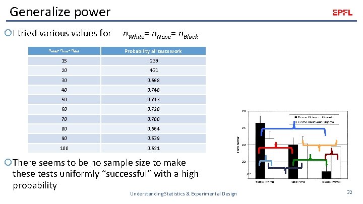
Generalize power I tried various values for n. White= n. None= n. Black Probability all tests work 15 . 239 20 . 431 30 0. 668 40 0. 748 50 0. 743 60 0. 728 70 0. 700 80 0. 664 90 0. 639 100 0. 621 There seems to be no sample size to make these tests uniformly “successful” with a high probability Understanding Statistics & Experimental Design 32

Generalize power For experimental design you want to consider all of the comparisons that matter for your theory The more constraints you impose on your dataset, the lower the probability any dataset will satisfy those constraints Simple theories are easier to test than complex theories In a complementary way, setting a criterion of p<. 05 is only for a particular test If you have multiple tests in a complex design, the probability of at least one test producing a Type I error is larger than. 05 Understanding Statistics & Experimental Design 33

Assumptions Common hypothesis tests t-tests, ANOVA Make assumptions about the population distributions Normal distribution Equal variances Make assumptions about sampling Fixed sample size What happens when these assumptions are violated? Not much in some situations Very bad things in some situations We mostly focus on control of the Type I error rate Understanding Statistics & Experimental Design 34

Normal distributions Simulated experiments for two-sample t tests with true null hypothesis https: //introstatsonline. com Log in with: ID=USEDF 16 -0, Password=epflstats Then navigate to https: //introstatsonline. com/chapters/chapter 12/homogeneity_variance_sim. shtml What if population distributions are not normal? Slight decrease in Type I error What if one population is normal and the other is not? Some increase in Type I error, especially if the non-normal population has a larger sample size Tends to disappear as sample sizes get larger As long as population distributions are approximately normal, then a t-test does a pretty good job controlling Type I error Understanding Statistics & Experimental Design 35

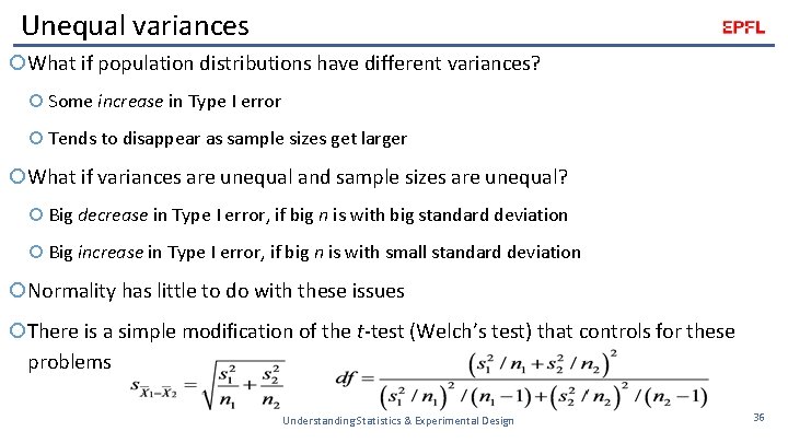
Unequal variances What if population distributions have different variances? Some increase in Type I error Tends to disappear as sample sizes get larger What if variances are unequal and sample sizes are unequal? Big decrease in Type I error, if big n is with big standard deviation Big increase in Type I error, if big n is with small standard deviation Normality has little to do with these issues There is a simple modification of the t-test (Welch’s test) that controls for these problems Understanding Statistics & Experimental Design 36

Sampling In general, larger samples are better for statistics More accurate measures of means, standard deviations, correlations More likely to reject the null if there is a true effect But the p value in hypothesis testing is based on the sampling distribution, which is typically defined for a fixed sample size If the sample size is not fixed, then the p value is not what it appears This has a number of effects Understanding Statistics & Experimental Design 37

Adding subjects Suppose you run a two-sample t-test with n 1=n 2=10 subjects You get p>. 05, but you want p<. 05 Many researchers add 5 new subjects to each group and repeat the test But you now have had two chances to reject the null. Even if the null is really true, the Type I error rate is now about 0. 08 Do this a second time and the Type I error rate is 0. 10 Do this a third time and the Type I error rate is 0. 12 Keep going up to a maximum sample size of n 1=n 2=50, and the Type I error rate is 0. 17 There is no need to add 5 subjects at a time. What if you just added 1 subject at a time to each group? Type I error rate is 0. 21 Sampling to a foregone conclusion! Understanding Statistics & Experimental Design 38

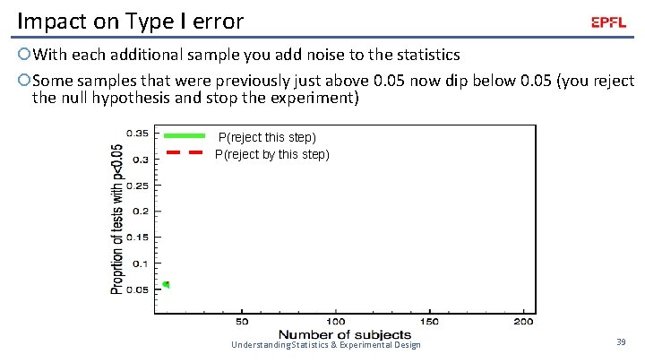
Impact on Type I error With each additional sample you add noise to the statistics Some samples that were previously just above 0. 05 now dip below 0. 05 (you reject the null hypothesis and stop the experiment) P(reject this step) P(reject by this step) Understanding Statistics & Experimental Design 39

Optional stopping The real problem is not with adding subjects, but with stopping when you like the outcome (e. g. , p<. 05) If you observe p=0. 03 and add more subjects, you might get p>. 05 This means that the interpretation of your p value depends on what you would do if you observed p<. 05 or p>. 05 If you would have added subjects when getting p>. 05, then even if you actually get p<. 05 you have an experimental method with an inflated Type I error rate If you do not know what you would have done, then you do not know the Type I error rate of your hypothesis test In fact, a given test does not have a Type I error rate, the error rate applies to the procedure not to a specific test Understanding Statistics & Experimental Design 40

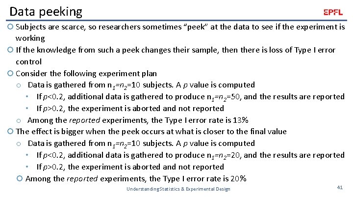
Data peeking Subjects are scarce, so researchers sometimes “peek” at the data to see if the experiment is working If the knowledge from such a peek changes their sample, then there is loss of Type I error control Consider the following experiment plan o Data is gathered from n 1=n 2=10 subjects. A p value is computed • If p<0. 2, additional data is gathered to produce n 1=n 2=50, and the results are reported • If p>0. 2, the experiment is aborted and not reported o Among the reported experiments, the Type I error rate is 13% The effect is bigger when the peek occurs at what is closer to the final value o Data is gathered from n 1=n 2=10 subjects. A p value is computed • If p<0. 2, additional data is gathered to produce n 1=n 2=20, and the results are reported • If p>0. 2, the experiment is aborted and not reported Among the reported experiments, the Type I error rate is 20% Understanding Statistics & Experimental Design 41

Conclusions Effect sizes Meta-analysis Power Hard to apply Needs to consider the full definition of experimental success Violations of hypothesis testing Minor effects for non-normal distributions Fixable effects for unequal variances Inflation of Type I error for non-fixed samples Understanding Statistics & Experimental Design 42

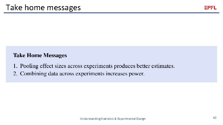
Take home messages Understanding Statistics & Experimental Design 43

END Class 9 Understanding Statistics & Experimental Design 44