Session 4 ANOVA Multiple Regression How to display

Session 4 - ANOVA & Multiple Regression

How to display means. Bars ok in simple situations 160 140 120 100 M 80 F 60 40 20 0 A B C D

Presenting means - ANOVA data One can also add “error bars” to these means. In analysis of variance, these error bars are based on the sample size and the pooled standard deviation, SDe. This SDe is the same residual SDe as in regression.

Don’t use bar graphs in complex situations 4

Use line graph 5

Fundamentals- comparing means

The “Yardstick” is critical

The “Yardstick” is critical yardstick: _____ 1 µm

The “Yardstick” is critical yardstick: _____ 10 meters

Weight loss comparison Diet mean weight loss (lbs) n Pritikin 5. 0 20 UCLA GS 9. 0 20 mean difference 4. 0 Is 4. 0 lbs a “big” difference? Compared to what? What is the “yardstick”?

The variation yardstick SD = 1, SEdiff=0. 32 , t=12. 6, p value < 0. 0001 12 Priticin 10 UCLA 8 6 4 2 0 0 3

The variation yardstick SD = 5 , SEdiff=1. 58, t= 2. 5, p value = 0. 02 35 30 25 Priticin 20 UCLA 15 10 5 0 -5 -10 -15 -20 0 3

Comparing Means Two groups – t test (review) Mean differences are “statistically significant” (different beyond chance) relative to their standard error (SEd) ____ t = (Y 1 - Y 2)= “signal” SE d “noise” _ Yi = mean of group i, SEd =standard error of mean difference t is mean difference in SEd units. As |t| increases, p value gets smaller. Rule of thumb: p < 0. 05 when |t| > 2 SEd is the “yardstick” for significance t & p value depend on: a) mean difference b) individual variability = SDs c) sample size (n)

How to compute SEd? SEd depends on n, SD and study design. (example: factorial or repeated measures) For a single mean, if n=sample size _ _____ SEM = SD/ n = SD 2/n __ For a mean difference (Y 1 - Y 2) The SE of the mean difference, SEd is given by _________ SEd = [ SD 12/n 1 + SD 22/n 2 ] or ________ SEd = [SEM 12 + SEM 22] If data is paired (before-after), first compute differences (di=Y 2 i-Y 1 i) for each person. For paired: SEd =SD(di)/√n

3 or more groups-analysis of variance (ANOVA) Pooled SDs What if we have many treatment groups, each with its own mean and SD? Group Mean SD sample size (n) A Y 1 SD 1 n 1 B Y 2 SD 2 n 2 C Y 3 SD 3 n 3 … __ k Yk SDk nk __

Variance (SD) homogeneity assumed true for usual ANOVA

The Pooled SDe the common yardstick SD 2 pooled error = SD 2 e = (n 1 -1) SD 12 + (n 2 -1) SD 22 + … (nk-1) SDk 2 (n 1 -1) + (n 2 -1) + … (nk-1) ____ so, SDe = SD 2 e

ANOVA uses pooled SDe to compute SEd and to compute “post hoc” (post pooling) t statistics and p values. __________ SEd = [ SD 12/n 1 + SD 22/n 2 ] ______ = SDe (1/n 1) + (1/n 2) SD 1 and SD 2 are replaced by SDe a “common yardstick”. If n 1=n 2=…=n, then SEd = SDe 2/n=constant

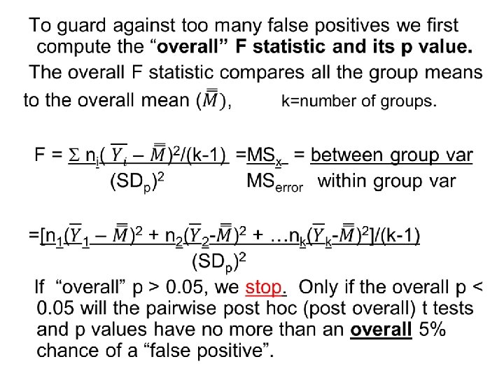
Multiplicity & F tests Multiple testing can create “false positives”. We incorrectly declare means are “significantly” different as an artifact of doing many tests even if none of the means are truly different from each other. Imagine we have k=four groups: A, B, C and D. There are six possible mean comparisons: A vs B A vs C A vs D B vs C B vs D C vs D

If we use p < 0. 05 as our “significance” criterion, we have a 5% chance of a “false positive” mistake for any one of the six comparisons, assuming that none of the groups are really different from each other. We have a 95% chance of no false positives if none of the groups are really different. So, the chance of a “false positive” in any of the six comparisons is 1 – (0. 95)6 = 0. 26 or 26%.

This criterion was suggested by RA Fisher and is called the Fisher LSD (least significant difference) criterion. It is less conservative (has fewer false negatives) than the very conservative Bonferroni criterion: if making “m” comparisons, declare significant only if p < 0. 05/m. This F test is an “omnibus” test.

F statistic interpretation F is the ratio of between group variation (variation across the means) relative to (pooled) within group variation. This is why this method is called “analysis of variance” Total variation = Variation between (among) the means (between group) + Pooled variation around each mean (within group) Between group variation Within group variation Total variation F = Between / Within F ≈ 1 -> not significant (R 2=Between variation/Total variation)

F distribution – under null

Ex: Clond-time to fall off rod (sec)

One way analysis of variance time to fall data, k= 4 groups, df= k-1 R square Adj R square 0. 5798 0. 5530 Root Mean Square Error=SDe Mean of Response Observations (or Sum Wgts) 10. 99 30. 20 51 Source DF Sum of Squares Mean Square group 3 7827. 438 2609. 15 Error 47 5672. 546 120. 69 Total 50 13499. 984 p value F Ratio Prob > F 21. 618 SDe 2 <. 0001

Means & SDs in sec (JMP) No model Level Number Mean median SD SEM KO-no TBI 8 21. 196 21. 65 6. 4598 2. 2839 KO-TBI 7 18. 659 18. 47 8. 7316 3. 3002 WT-no. TBI 15 49. 197 46. 93 9. 9232 2. 5622 WT-TBI 21 23. 902 23. 33 13. 3124 2. 9050 ANOVA model, pooled SDe=10. 986 sec Level Number Mean SEM KO-no TBI 8 21. 196 3. 8841 KO-TBI 7 18. 659 4. 1523 WT-no. TBI 15 49. 197 2. 8366 WT-TBI 21 23. 902 2. 3973 Why are SEMs not the same? ?

Mean comparisons- post hoc t Level WT-no. TBI Mean A 49. 197 WT-TBI B 23. 902 KO-no TBI B 21. 196 KO-TBI B 18. 659 Means not connected by the same letter are significantly different

Multiple comparisons-Tukey’s q As an alternative to Fisher LSD, for pairwise comparisons of “k” means, Tukey computed percentiles for q=(largest mean-smallest mean)/SEd under the null hyp that all means are equal. If mean diff > q SEd is the significance criterion, type I error is ≤ α for all comparisons. q > t > Z One looks up ”t” on the q table instead of the t table.

t or Z (unadjusted) vs q (Tukey)– 3 means

t (or Z) vs q for α=0. 05, large n num means=k t q* 2 1. 96 3 1. 96 2. 34 4 1. 96 2. 59 5 1. 96 2. 73 6 1. 96 2. 85 * Some tables give q for SE, not SEd, so must multiply q by √ 2.

Post hoc: t vs Tukey q, k=4 Level vs Level Mean Diff SE diff t p-Value- no correction p-Value. Tukey WT-no. TBI KO-TBI 30. 54 5. 03 6. 073 <. 0001* WT-no. TBI KO-no TBI 28. 00 4. 81 5. 822 <. 0001* WT-no. TBI WT-TBI 25. 30 3. 71 6. 811 <. 0001* WT-TBI KO-TBI 5. 24 4. 79 1. 094 0. 2797 0. 6952 WT-TBI KO-no TBI 2. 71 4. 56 0. 593 0. 5562 0. 9338 KO-no TBI KO-TBI 2. 54 5. 69 0. 446 0. 6574 0. 9700

Mean comparisons-Tukey Level WT-no. TBI Mean A 49. 197 WT-TBI B 23. 902 KO-no TBI B 21. 196 KO-TBI B 18. 659 Means not connected by the same letter are significantly different

Transformations There are two requirements for the analysis of variance (ANOVA) model. 1. Within any treatment group, the mean should be the middle value. That is, the mean should be about the same as the median. When this is true, the data can usually be reasonably modeled by a Gaussian (“normal”) distribution. 2. The SDs should be similar (variance homogeneity) from group to group. Can plot mean vs median & residual errors to check #1 and mean versus SD to check #2.

What if its not true? Two options: a. Find a transformed scale where it is true. b. Don’t use the usual ANOVA model (use non constant variance ANOVA models or non parametric models). Option “a” is better if possible - more power.

Most common transform is log transformation Usually works for: 1. Radioactive count data 2. Titration data (titers), serial dilution data 3. Cell, bacterial, viral growth, CFUs 4. Steroids & hormones (E 2, Testos, …) 5. Power data (decibels, earthquakes) 6. Acidity data (p. H), … 7. Cytokines, Liver enzymes (Bilirubin…) In general, log transform works when a multiplicative phenomena is transformed to an additive phenomena.

Compute stats on the log scale & back transform results to original scale for final report. Since log(A)–log(B) =log(A/B), differences on the log scale correspond to ratios on the original scale. Remember 10 mean(log data) =geometric mean < arithmetic mean monotone transformation ladder- try these Y 2, Y 1. 5, Y 1, Y 0. 5=√Y, Y 0=log(Y), Y-0. 5=1/√Y, Y-1=1/Y, Y-1. 5, Y-2

Multiway ANOVA

Balanced designs - ANOVA example Brain Weight data, n=7 x 4 = 28, nc=7 obs/cell Dementia Sex Brain Weight (gm) No No … F F F F … 1223 1228 1222 1204 1234 1211 1217 …

Terminology – cell means, marginal means Males Females Overall Dementia Cell Margin No dementia Cell Margin Overall Margin

Mean brain weights (gms) in Males and Females with and without dementia A balanced* 2 x 2 (ANOVA) design, nc= 7 obs per cell, n=7 x 4 = 28 obs total Means Cell mean Males (1) Female (-1) Margin Yes (1) 1321. 14 1201. 71 1261. 43 No (-1) 1333. 43 1219. 86 1276. 64 Margin 1327. 29 1210. 79 1269. 04 Dementia

Brain weight, n=7 x 4 = 28 Difference in marginal sex means (Male – Female) 1327. 29 - 1210. 79 = 116. 50, 116. 50/2 = 58. 25 Difference in marginal dementia means (Yes – No) 1261. 43 - 1276. 64 = -15. 21, -15. 21/2 = -7. 61 Difference in cell mean differences-interaction (1321. 14 - 1333. 43) – (1201. 71 - 1219. 86) = 5. 86 (1321. 14 - 1201. 71) – (1333. 43 - 1219. 86) = 5. 86 note: 5. 86/(2 x 2) = 1. 46 Parallel (additive) when interaction is zero * balanced = same sample size (nc) in every cell

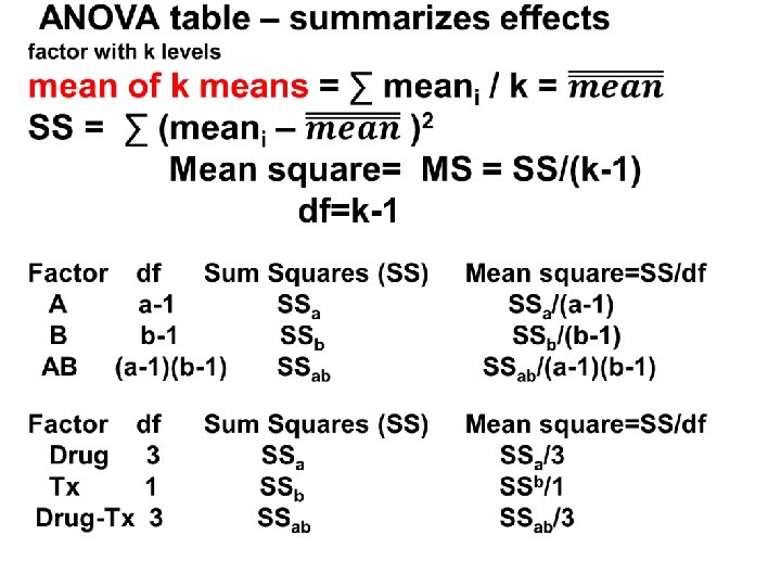
Brain weight ANOVA MODEL: brain wt = sex, dementia , sex*dementia Class Levels Values sex 2 -1 1 dementia 2 -1 1 n=28 observations, n c=7 per cell Source DF Sum of Squares Mean Square F Value p value Model 3 96686 32228. 70 451. 05 <. 0001 Error 24 1715 71. 45 = SD 2 e C Total 27 98402 R-Square Coeff Var Root MSE Mean brain wt 0. 9826 0. 666092 8. 453=SDe 1269. 04 ANOVA table – summarizes effect of each factor Source DF SS Mean Square F Value p value sex 1 95005. 75 1329. 64 <. 0001 dementia 1 1620. 32 22. 68 <. 0001 sex*dementia 1 60. 04 0. 84 0. 3685 SS= n (mean diff)2 n=28 Sex 58. 252 x 28 = 95005. 75 Dementia 7. 612 x 28 = 1620. 32 Sex-dementia 1. 462 x 28 = 60. 04

Mean brain wt vs dementia & sex parallel = no interaction

ANOVA intuition Y may depend on group (A, B, C), sex & their interaction. Which is significant in each example?

ANOVA intuition (cont)

Example: 4 x 2 Design Treatment Control Drug margin Drug A Cell mean Marginal mean Drug B Cell mean Marginal mean Drug C Cell mean Marginal mean Drug D Cell mean Marginal mean Grand mean

Multiway ANOVA example Wish to evaluate influence of: Gender (M or F) – 2 levels Race/Ethnicity (A, B, H, W) – 4 levels Education (no HS, BA, MA, Ph. D) – 5 levels Occupation (laborer, office worker, manager, scientist, health worker) – 5 levels on Y = depression score Y has a normal distribution. 2 x 4 x 5 = 200 combinations (cells)

Why is the ANOVA table useful? Dependent Variable: depression score Source DF SS Mean Square F Value overall p value Model 199 3387. 41 17. 02 4. 42 <. 0001 Error 400 1540. 17 3. 85 Corrected Total 599 4927. 58 root MSE=1. 962=SDe, R 2=0. 687 Source DF SS Mean Square F Value p value gender 1 778. 084 202. 08 <. 0001 race 3 229. 689 76. 563 19. 88 <. 0001 educ 4 104. 838 26. 209 6. 81 <. 0001 occ 4 1531. 371 382. 843 99. 43 <. 0001 gender*race 3 1. 879 0. 626 0. 16 0. 9215 gender*educ 4 3. 575 0. 894 0. 23 0. 9203 gender*occ 4 8. 907 2. 227 0. 58 0. 6785 race*educ 12 69. 064 5. 755 1. 49 0. 1230 race*occ 12 62. 825 5. 235 1. 36 0. 1826 educ*occ 16 60. 568 3. 786 0. 98 0. 4743 gender*race*educ 12 77. 742 6. 479 1. 68 0. 0682 gender*race*occ 12 59. 705 4. 975 1. 29 0. 2202 gender*educ*occ 16 100. 920 6. 308 1. 64 0. 0565 race*educ*occ 48 206. 880 4. 310 1. 12 0. 2792 gender*race*educ*occ 48 91. 368 1. 903 0. 49 0. 9982

8 graphs of 200 depression means. Y=depr, X=occ (occupation), X=educ. separate graph for each gender & race Males Females W W B B H H A A

One of the 8 graphs Note parallelism implying no interaction

Evaluating the ANOVA table Wish to determine which “main effects” and interactions to retain. Start at bottom of table with the highest order (most complicated) interaction (gender*race*educ*occ). If this interaction is not significant, can remove. Then recalculate p values for remaining terms after interaction removed as the p values can change. Keep removing until all remaining terms are significant.

Hierarchy rule for interactions When evaluating interactions, cannot remove “non significant” lower order (simpler) interaction unless corresponding higher order interaction is also not significant and is removed first. Example: (main effects A, B, C not shown) Factor p value A*B 0. 7149 A*C 0. 0234 B*C 0. 4479 A*B*C < 0. 0001 Although A*B and B*C are not significant, can’t remove A*B or B*C since A*B*C is significant and contains B.

Depression-final model Sum of Source DF Squares Mean Square F overall p Model 12 2643. 981859 220. 331822 56. 64 <. 0001 Error 587 2283. 610408 3. 89030=SDe 2 Corrected Total 599 4927. 592267 R-Square Coeff Var Root MSE y Mean 0. 536567 21. 24713 1. 972386=SDe 9. 283069 Source DF SS Mean Square F Value p value gender 1 778. 084257 778. 08 200. 01 <. 0001 race 3 229. 688698 76. 56 19. 68 <. 0001 educ 4 104. 837607 26. 21 6. 74 <. 0001 occ 4 1531. 371296 382. 84 98. 41 <. 0001 Analysis shows that factors are additive (no significant interactions)

Marginal means-depression

If one of the factors is NOT significant, the entire set of means for that factor can be collapsed. The "sum of squares" ANOVA table is a summary table that is useful for screening, particularly screening interactions. It allows one to test "chunks" of the model. If we also have balance, then all the parts above are orthogonal (uncorrelated) so the assessment of one factor or interaction is not affected if another factor or interaction is significant or not. This is an ideal analysis situation but is not common.

If all of the interaction terms are NOT significant, then one has proven that the influence of all the factors on the outcome Y is additive. If all the interaction terms for factor “B” are not significant, then the impact of factor B on Y is additive. Must follow the hierarchical rule: Cannot remove lower order interaction involving factor “B” unless all higher order interactions with B are not significant.

Regression – Associations via equations

Example: apnea risk calculator How many hours of sleep do you get: a. 5 or less (15 pts), b. 6 -8 (0 pts) , c. 9+ (5 pts) What best describes your sleeping pattern: a. sound sleep all night (0 pts) b. wake up once and go back to sleep (5 pts) c. wake up multiple times & go back to sleep (10 pts) d. wake up and cannot get back to sleep (15 pts) Do you snore: a. No (0 pts) b Yes (10 pts)

Multiple Regression - Overview Multiple Regression in statistics is the science and art of creating an equation that relates an outcome Y, to one or more predictors, X 1, X 2, X 3, . . Xk. Linear Regression Y = a + b 1 X 1 + b 2 X 2 + b 3 X 3 +. . . + bk Xk + e = Ŷ + e where the “b”s are the weights and "e" is the residual error between the observed Y and the prediction (Ŷ). In linear regression, bi is the average change in Y for a single unit change in Xi. “Performance” stats: R 2, SDe

Predictors of Y=SBP in children Gilman et. al. JAMA, v 267, no 17, May 1992 SBP= -9. 20 -2. 27 Ca + 4. 03 sex + 0. 25 Ht + 2. 02 BMI + 0. 51 HR = error

Logistic Regression In multiple logistic regression, Y is 0 or 1 with mean P, the “risk”. The logit of P, not P, is assumed a linear function of the Xs Logit(P) = ln(P/(1 -P)) = a + b 1 X 1 + b 2 X 2 + b 3 X 3 +. . . + bk Xk (“Logit” = log of the odds since P/(1 -P) is the odds) odds=exp(a + b 1 X 1 + b 2 X 2 + b 3 X 3 +. . . + bk Xk) risk = P = odds/(odds+1) “Performance” stats: Sensitivity, Specificity, Accuracy, Concordance (C), mean deviance Poisson Regression When Y is a positive integer (0, 1, 2, 3…), we model the log of Y so Y can never be negative. This is the multiple Poisson regression model. ln(mean Y) = a + b 1 X 1 + b 2 X 2 + b 3 X 3 +. . . + bk Xk mean Y = exp(a + b 1 X 1 + b 2 X 2 + b 3 X 3 +. . . + bk Xk) mean Y cannot be negative. “Performance” stats: R 2, mean deviance

Logit function: logit=ln(P/(1 -P)) vs P

Logistic regression Predictors of in hospital infection Characteristic Odds Ratio (95% CI) p value Incr APACHE score 1. 15 (1. 11 -1. 18) <. 001 Transfusion (y/n) 4. 15 (2. 46 -6. 99) <. 001 Increasing age (yr) 1. 03 (1. 02 -1. 05) <. 001 Malignancy 2. 60 (1. 62 -4. 17) <. 001 Max Temperature 0. 70 (0. 58 -0. 85) <. 001 Adm to treat>7 d 1. 66 (1. 05 -2. 61) 0. 03 Female (y/n) 1. 32 (0. 90 -1. 94) 0. 16 *APACHE = Acute Physiology & Chronic Health Evaluation Score

Multiple Proportional Hazards Regr (Cox model) For time dependent outcomes (ie time to death), we model the hazard rate, h , the event rate per unit time (for death, it is the mortality rate). Since h > 0, we model the log of the hazard as a linear function of the Xs so h can never be zero (similar to Poisson regression). ln(h) = a + b 1 X 1 + b 2 X 2 + b 3 X 3 +. . . + bk Xk so h = exp(a + b 1 X 1 + b 2 X 2 + b 3 X 3 +. . . + bk Xk) > 0 If h 0=exp(a) is the ‘baseline’ hazard, (that is, a=log(h 0)) the hazard ratio is HR = h/h 0 = exp(b 1 X 1 + b 2 X 2 + b 3 X 3 +. . . + bk Xk) no intercept ‘a’. If S 0(t) is the ‘baseline’ survival curve corresponding to the baseline hazard, then the survival curve for a given combination of X 1, X 2, … Xk is given by S(t) = S 0(t)HR where HR is computed with the equation above. exp(bi) is the hazard rate ratio for a one unit change in Xi. “Performance” stats: Harrell’s Concordance (C) (0. 5 < C < 1. 0)

Cox regr-HR for patient mortality- Busuttil et al 2005

Cox HRs for donor age (Busuttil 2005) Donor age HR 95% CI p value 1 -18 1. 00 (ref) -- -- 18 -32 1. 23 0. 88 -1. 72 0. 20 32 -48 1. 40 1. 02 -1. 92 0. 03 48 -55 1. 51 1. 02 -2. 24 0. 04 55 -60 2. 29 1. 48 -3. 55 < 0. 001 60+ 1. 61 1. 10 -2. 37 0. 01 Harrell C= 0. 70

Regression coeff interpretation Outcome (Y) Regression interpretation continuous Linear b is the average change in Y per one unit increase in X, the rate of change Binary Logistic exp(b)=eb=odds ratio (OR) for a one unit increase in X Low Positive integers (0, 1, 2, 3. . ) Poisson exp(b)= mean ratio (MR) for a one unit increase in X Hazard rate Cox exp(b)=hazard rate ratio (HR) for a one unit increase in X (P=proportion) (h=events/time) S(t) = S 0(t)HR

Multiple Linear Regression Example Consider predictors of Y=Bilirubin (mg/dl) in liver transplant candidates. Two predictors are X 1=Prothombin time (PT) in seconds X 2=ALT (alanine aminotransferase in U/L). A multiple regression equation (on the log scale) is Ŷ = (predicted) log Bilirubin = -3. 96 + 3. 47 log PT + 0. 21 log ALT

Regression output - equation (Equation) Parameter estimates term estimate SE t ratio p value Intercept -3. 96 0. 257 -15. 4 < 0. 001 log PT 3. 47 0. 214 16. 2 < 0. 001 log ALT 0. 21 0. 055 3. 8 0. 0002 equation: Log Bili=-3. 96 + 3. 47 log PT + 0. 21 log ALT

Interpreting multiple regression coefficients (cont. ) The multiple regression coefficients will not in general be the same as the individual regression coefficient for each variable one at a time, even though the same Y is being modeled. Simple regression Multiple (simultaneous) variable (one Y, one X) (b 1 X 1+b 2 X 2) Log PT 3. 560 3. 470 Log ALT 0. 310 0. 211 Log Bilirubin = - 3. 70 + 3. 56 log PT, R 2 = 0. 425 Log Bilirubin = -. 105 + 0. 310 log ALT, R 2 = 0. 049 Log PT coefficients don’t match Log Bilirubin = -3. 96 + 3. 47 log PT + 0. 211 log ALT , R 2 = 0. 448

Orthogonally (vs collinearity) In general, regression coefficients from simple and multiple regression are not the same ↔ controlling for covariates does not give the same answer as ignoring covariates. Only when all the X variables have correlation zero with each other will the simple and multiple regression coefficients be the same orthogonally (Collinearity is when Xs are strongly correlated. It is the “opposite” of orthogonality).

Log PT (X 1) vs log ALT (X 2) since correlation is low, unadjusted and adjusted regression results are similar r 12 = 0. 111, R 2 = 0. 0123

CESD depression-bivariate Scale 0 -50 variable sex (F-M) age (per yr)* Unemploy (vs other) income (per 1000)* drink (yes vs no) health (poor-non poor) regdoc (yes vs no) beddays (yes vs no) acuteill (yes vs no) chronill (yes vs no) slope (b) or mean difference 2. 24 -0. 080 6. 87 -0. 091 -0. 17 4. 55 -3. 74 5. 68 2. 04 1. 62 R 2 1. 5% 2. 7% 2. 6% 2. 5% 0. 1% 1. 2% 2. 7% 7. 0% 1. 1% 0. 8% total 22. 3% p value 0. 0342 0. 0048 0. 0043 0. 0066 0. 8967 0. 0598 0. 0044 < 0. 001 0. 0701 0. 1151 * Assume linear 75

CESD depression-multivariable all variables used green=bivariate Variable Intercept Estimate 13. 33 SE 2. 29 t Ratio 5. 81 p value 0. 0000 estimate p value sex-F age unemploy income 1. 20 -0. 082 4. 76 -0. 094 1. 03 0. 030 2. 30 0. 033 1. 16 -2. 76 2. 07 -2. 84 0. 2456 0. 0061 0. 0397 0. 0048 2. 24 -0. 080 6. 87 -0. 091 0. 0342 0. 0048 0. 0043 0. 0066 drink health-poor regdoc beddays acuteill chronill 0. 633 3. 71 -2. 46 4. 48 -0. 53 1. 30 1. 232 2. 41 1. 26 1. 35 1. 18 1. 03 0. 51 1. 54 -1. 94 3. 31 -0. 45 1. 25 0. 6080 0. 1244 0. 0528 0. 0010 0. 6529 0. 2111 -0. 17 4. 55 -3. 74 5. 68 2. 04 1. 62 0. 8967 0. 0598 0. 0044 < 0. 001 0. 0701 0. 1151 R square=16. 7%

CESD depression-final selected variables (backward stepwise, p < 0. 10) variable Estimate SE t Ratio p value Intercept 14. 69 1. 83 8. 03 0. 0000 age -0. 07 0. 03 -2. 57 0. 0107 unemploy 4. 62 2. 29 2. 01 0. 0449 income -0. 10 0. 03 -3. 13 0. 0019 health-poor 4. 03 2. 34 1. 72 0. 0866 regdoc -2. 31 1. 26 -1. 84 0. 0672 beddays 4. 68 1. 21 3. 87 0. 0001 R square=15. 6%

Interaction Effects & subgroups The model Y = 0 + 1 X 1 + 2 X 2 + implies that change in Y due to X 1 (= 1) is the same (constant) for all values of X 2. An ADDITIVE model. In the model Y = 0 + 1 X 1 + 2 X 2 + 3 X 1 X 2 + the 3 term is an interaction term. Change in Y for a unit change in X 1 is ( 1+ 3 X 2) and is therefore not constant. Positive 3 is often termed a “synergism” Negative 3 is often termed an “antagonism” Additive only if β 3=0 How to implement? Make new variable W = X 1 X 2.

Interaction example Response: Y= log HOMA IR (MESA study) R 2=0. 280, Root Mean Square Error=SDe=0. 623 Mean Response= 0. 395, n= 6782 Parameter Estimates Term Estimate Std Error t Ratio p value Intercept -1. 388 0. 049 -28. 16 <. 0001 Gender -0. 669 0. 085 -7. 83 <. 0001 BMI 0. 061 0. 00168 36. 45 <. 0001 gender*BMI 0. 028 0. 00299 9. 38 <. 0001 Predicted log HOMA IR = -1. 39 – 0. 669 gender + 0. 061 BMI + 0. 028 gender * BMI (gender is coded 0 for female and 1 for male)

gender x BMI interaction- non additivity In Females Log HOMA IR = -1. 39 +0. 061 BMI In Males Log HOMA IR = -2. 06 + 0. 089 BMI

Gender x BMI interaction relation is different in males vs females

Adjusted means

Ex: Meditation & change in pct body fat Overweight persons chose a meditation program or a “sham” (lectures) as part of a weight loss effort. They were NOT randomized. Change in percent body fat by treatment group (mediation or sham) over three months Unadjusted Means Level n Mean pct body SEM Mean dietary fat (gm) fat change (before study start) 1 -meditate 439 -7. 51% 0. 47% 32. 7 g 2 -sham 704 1. 34% 0. 35% 67. 1 g Unadjusted Mean difference (sham - meditation) = 8. 85% SE of the difference = SEd = √ 0. 47222 + 0. 35322 = 0. 59% t = mean diff/SEd = 8. 85% / 0. 59% = 15. 1, p < 0. 0001 Overall unweighted dietary fat = 49. 9 g

Result via “regression” Y= change in body fat, X = 1 if sham, 0 if meditation Y = a + b X + error = a + b sham + error term estimate SE t p value a -7. 51 0. 46 -16. 4 < 0. 001 b 8. 85 0. 59 15. 2 < 0. 001 Ŷ = -7. 51 + 8. 85 sham

Regr-control for dietary fat pct body fat= Y = a + b 1 X 1 + b 2 X 2 + error X 1= 1 if sham, 0 if meditation X 2 = dietary fat in g term estimate SE t p value a -14. 5 0. 54 -26. 6 < 0. 001 b 1 1. 51 0. 56 2. 7 0. 007 b 2 0. 21 0. 011 18. 9 <0. 001 body fat chg=-14. 5 +1. 51 sham +0. 21 diet fat

Adjusted means Plug into equation for X 1=1=sham or X 1=0. Hold X 2 = diet fat= 49. 9 g – overall mean X 2 Med: -14. 5 + 1. 51(0)+0. 213(49. 9)=-3. 84% Sham: -14. 5 + 1. 51(1)+0. 213(49. 9)=-2. 33% Adj mean difference =2. 33 -(-3. 84) =1. 51% (Unadjusted was 8. 85%)

General procedure Adjusted means for X 1, controlling for (confounders) X 2, X 3, X 4 … 1. Estimate model regression coefficients 2. Plug in different values for X 1, and values for all other Xs held constant at their overall means. Gives adjusted means and their SEs. Assumes ? ?