The Monte Carlo Method an Introduction Detlev Reiter

The Monte Carlo Method: an Introduction Detlev Reiter Research Centre Jülich (FZJ) D -52425 Jülich http: //www. fz-juelich. de e-mail: d. reiter@fz-juelich. de Tel. : 02461 / 61 -5841 Vorlesung HHU Düsseldorf, WS 07/08 March 2008

There are two dominant methods of simulation for complex many particle systems 1) Molecular Dynamics • • Solve the classical equations of motion from mechanics. Particles interact via a given interaction potential. Deterministic behaviour (within numerical precision). Find temporal evolution. 2) Monte Carlo Simulation • • Find mean values (expectation values) of some system components. Random behaviour from given probability distribution laws. The Monte Carlo technique is a very far spread technique, because it is not limited to systems of particles.

This lecture • Brief introduction: simulation • What is the Monte Carlo Method • Random number generation • Integration by Monte Carlo Tomorrow: one (of many) particular application: • particle transport by Monte Carlo

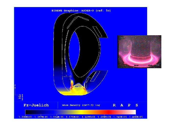
ASDEX-UPDRADE (IPP Garching) 4

Monte Carlo particle trajectories, ions and neutral particles

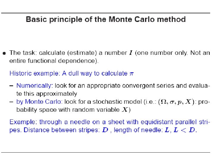
First application of Monte Carlo Method The needle experiment of Compte de Buffon, 1733 (french biologist, 1707 -1788 What is the probability p, that a needle (length L), which randomly falls on a sheet, crosses one of the lines (distance D)? (N trials, n „hits“)

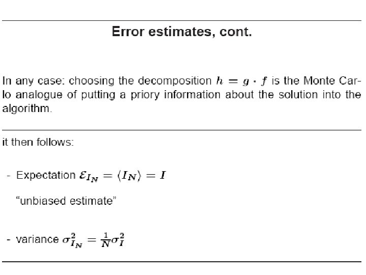
Yt =1, if crossing, Yt=0 else, then

Today: Using a computer to generate random events: We need to be able to generate random numbers X with any given probability function f(x), or a given cumulative distribution F(x). 1) Uniformly distributed random numbers 2) General random numbers: can be obtained from a sequence of independent uniform random numbers

Random number generation f(x) 1/(b-a) a b

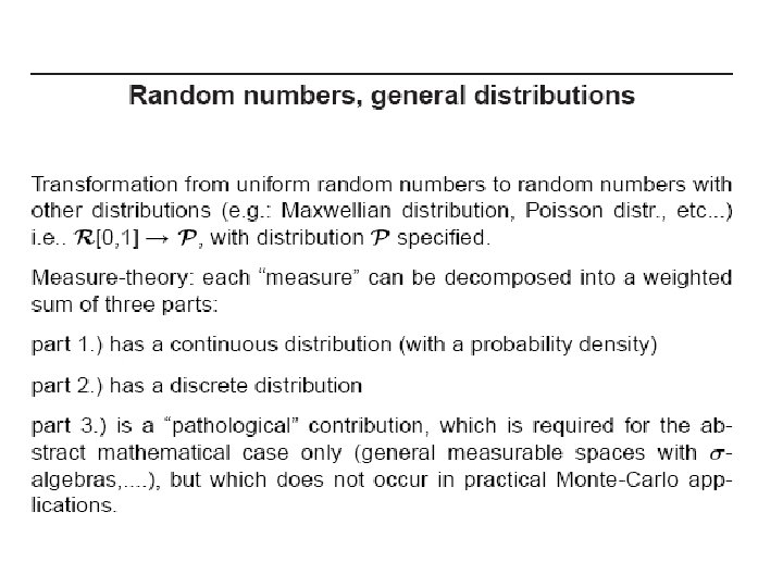
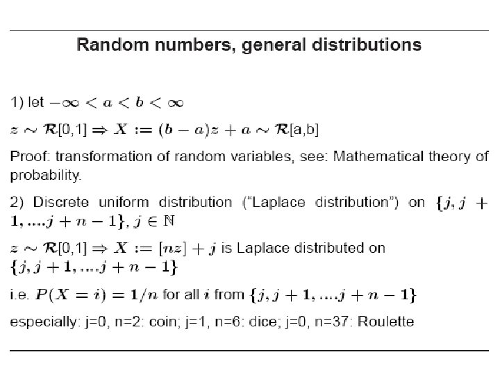
We will see next: Any continuous distribution can be generated from uniform random numbers on [0, 1] Any discrete distribution can be generated from uniform random numbers on [0, 1] Hence: Any given distribution can be generated from uniform random numbers on [0, 1]

Strategy: try to transform F to another distribution, such that inverse of new F is explicitly known.

Example: Normal (Gaussian) distribution Cumulative distr. function Inverse cumul. distr. fct. best format of storing distributions for Monte Carlo applications: „Inverse cumulative distribution function F-1(x)“, x uniform [0, 1]

Exercise (and most important example: ) Generate random numbers from a Gaussian. Let X, Y two independent Gaussian random numbers. Transform to polar coordiantes (Jacobian!) R, Φ Sample Φ (trivial, it is uniform on 2π) Apply inversion method for R Transform sampled Φ, R back to X, Y. This is a pair of Gaussians. (Box-Muller Method)

Exponential distribution by „inversion“ Note: Z and 1 -Z have same distrib. (see tomorrow)

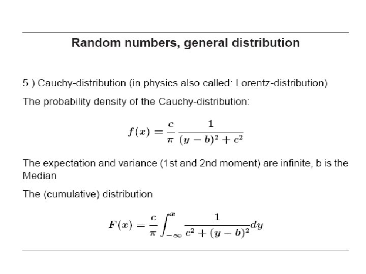
Cauchy: e. g. : natural Line broadening

(stepwise constant, with steps at points T)

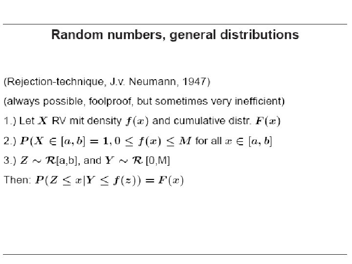
Rejection y=f(x): distribution density enclosing rectangle Reject z Accept z, take x=z y uniform sample x from f(x) X z, uniform

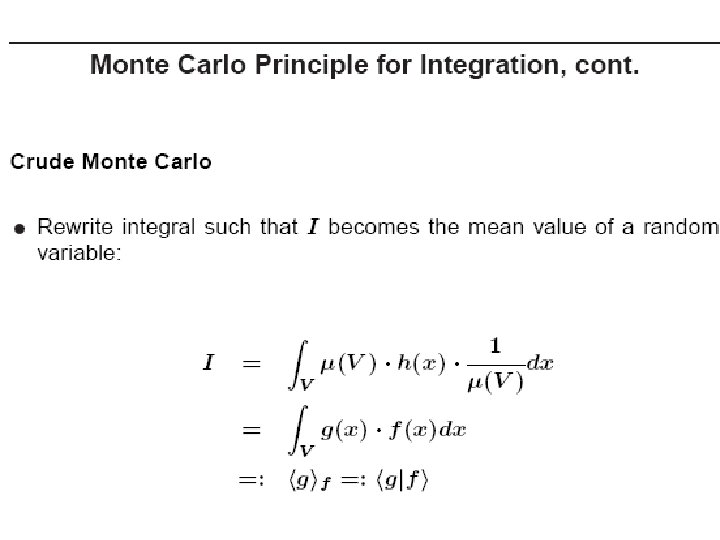
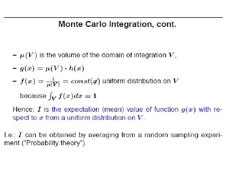
NEXT: Any Monte Carlo estimate can be regarded as a mean value, i. e. an integral (or sum) over a given probability distribution, ususally in a high dimensional space (e. g. of random walks…. ) Generic Monte Carlo: Integration Hence: How does Monte Carlo integration work?

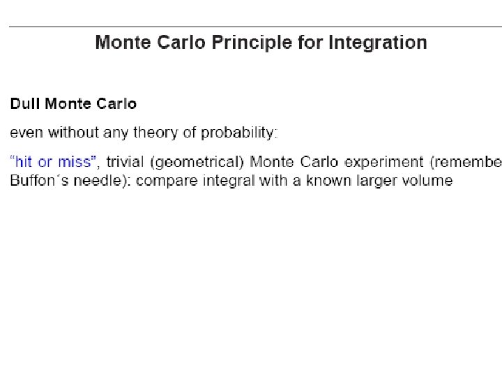
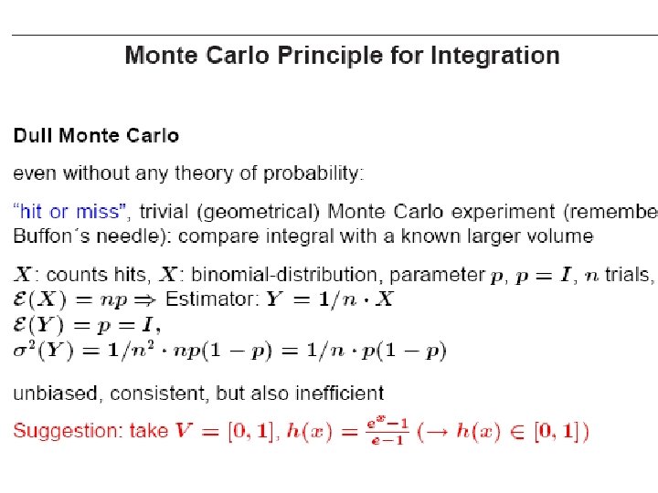
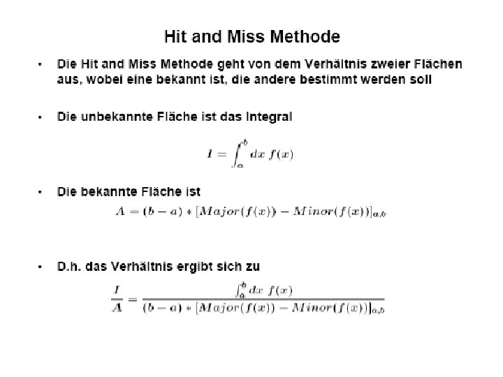
Hit or Miss f(x) x 2 uniform I: unknown area miss hit I = ∫ f(x) dx X x 1, uniform

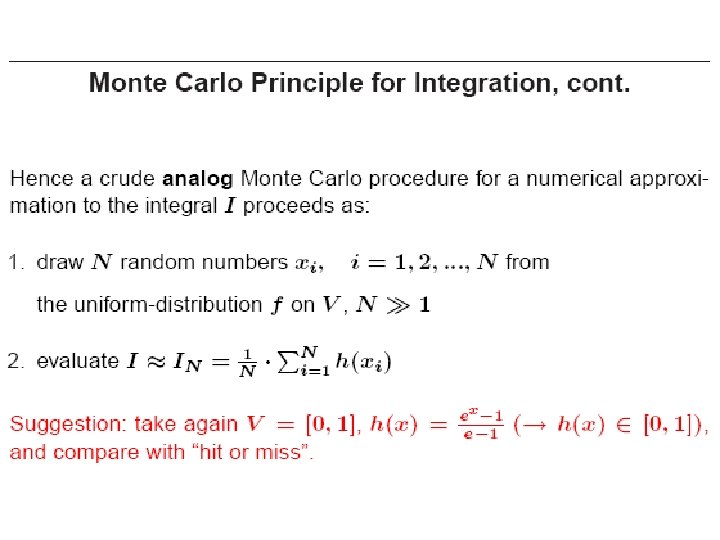
Suggestion: try again with previous example from dull and crude Monte Carlo

Outlook: next lecture (tomorrow)

END