Stochastic Local Search Computer Science cpsc 322 Lecture

(Stochastic) Local Search Computer Science cpsc 322, Lecture 5 (Textbook Chpt 4. 8 -4. 9) May, 22, 2012 CPSC 322, Lecture 5 Slide 1

Course Announcements Posted on Web. CT • Assignment 2 on CSPs (due on Thurs!) If you are confused about basic CSPs…. . Check learning goals at the end of lectures. Please come to office hours • Work on CSPs Practice Ex: • Exercise 4. A: arc consistency • Exercise 4. B: constraint satisfaction problems • Exercise 4. C: SLS for CSP • MIDTERM: Mon May 28 th – 3 PM (room TBA) CPSC 322, Lecture 5 Slide 2

Systematically solving CSPs: Summary • Build Constraint Network • Apply Arc Consistency • One domain is empty • Each domain has a single value • Some domains have more than one value • Apply Depth-First Search with Pruning • Split the problem in a number of disjoint cases • Apply Arc Consistency to each case CPSC 322, Lecture 5 Slide 3

Local Search motivation: Scale • Many CSPs (scheduling, DNA computing, more later) are simply too big for systematic approaches • If you have 105 vars with dom(vari) = 104 • Systematic Search • Constraint Network • but if solutions are densely distributed……. CPSC 322, Lecture 5 Slide 4

Lecture Overview • Local search • Constrained Optimization • Greedy Descent / Hill Climbing: Problems • Stochastic Local Search (SLS) • Comparing SLS algorithms • SLS variants üTabu lists üSimulated Annealing • Population Based üBeam search üGenetic Algorithms CPSC 322, Lecture 5 Slide 5

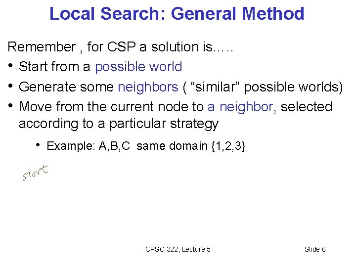
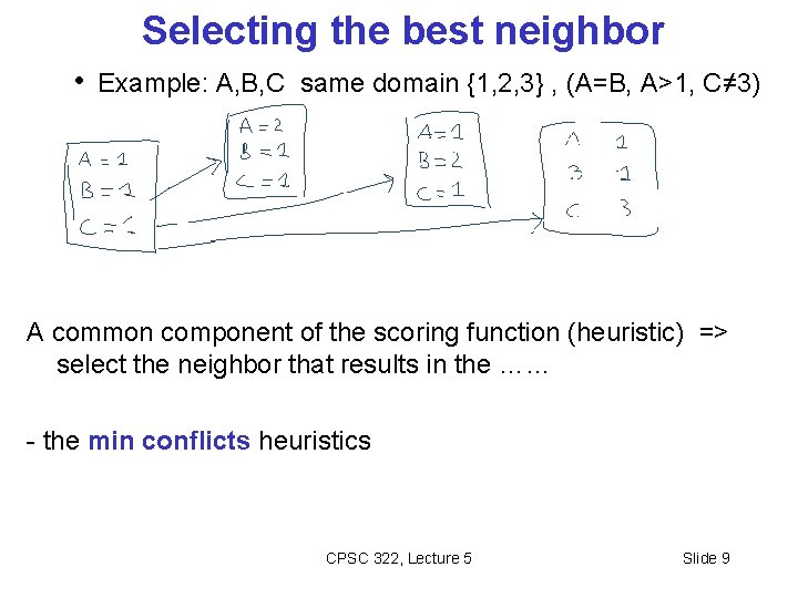
Local Search: General Method Remember , for CSP a solution is…. . • Start from a possible world • Generate some neighbors ( “similar” possible worlds) • Move from the current node to a neighbor, selected according to a particular strategy • Example: A, B, C same domain {1, 2, 3} CPSC 322, Lecture 5 Slide 6

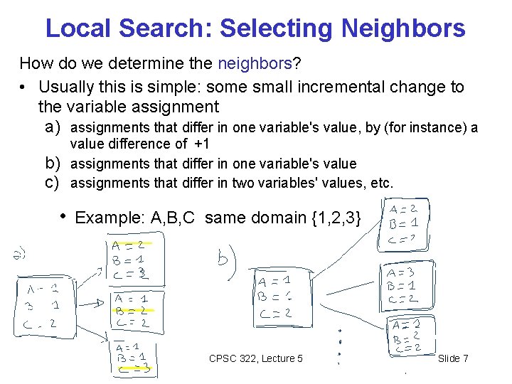
Local Search: Selecting Neighbors How do we determine the neighbors? • Usually this is simple: some small incremental change to the variable assignment a) assignments that differ in one variable's value, by (for instance) a b) c) value difference of +1 assignments that differ in one variable's value assignments that differ in two variables' values, etc. • Example: A, B, C same domain {1, 2, 3} CPSC 322, Lecture 5 Slide 7

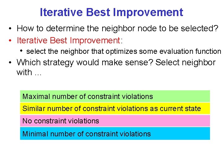
Iterative Best Improvement • How to determine the neighbor node to be selected? • Iterative Best Improvement: • select the neighbor that optimizes some evaluation function • Which strategy would make sense? Select neighbor with … Maximal number of constraint violations Similar number of constraint violations as current state No constraint violations Minimal number of constraint violations

Selecting the best neighbor • Example: A, B, C same domain {1, 2, 3} , (A=B, A>1, C≠ 3) A common component of the scoring function (heuristic) => select the neighbor that results in the …… - the min conflicts heuristics CPSC 322, Lecture 5 Slide 9

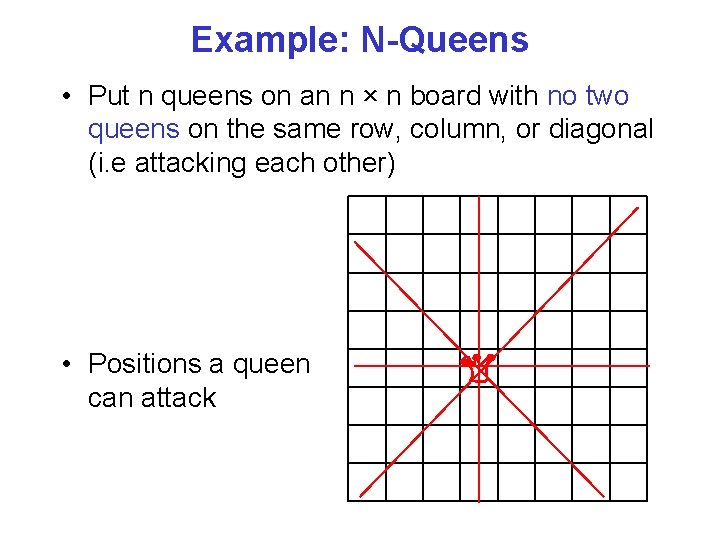
Example: N-Queens • Put n queens on an n × n board with no two queens on the same row, column, or diagonal (i. e attacking each other) • Positions a queen can attack

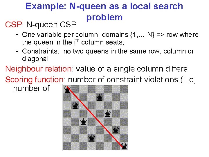
Example: N-queen as a local search problem CSP: N-queen CSP - One variable per column; domains {1, …, N} => row where - the queen in the ith column seats; Constraints: no two queens in the same row, column or diagonal Neighbour relation: value of a single column differs Scoring function: number of constraint violations (i. . e, number of attacks)

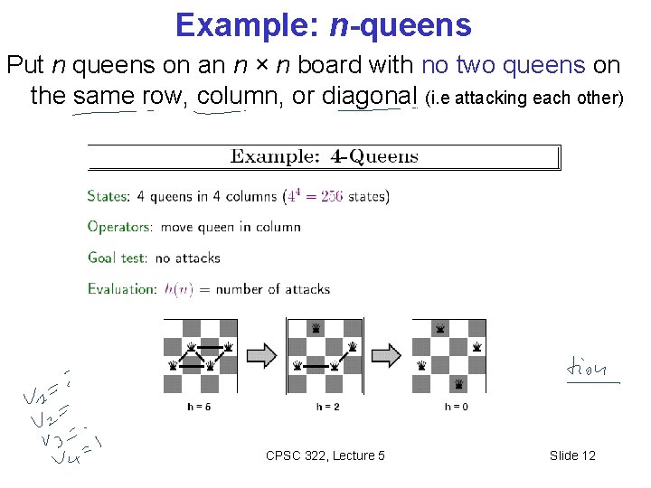
Example: n-queens Put n queens on an n × n board with no two queens on the same row, column, or diagonal (i. e attacking each other) CPSC 322, Lecture 5 Slide 12

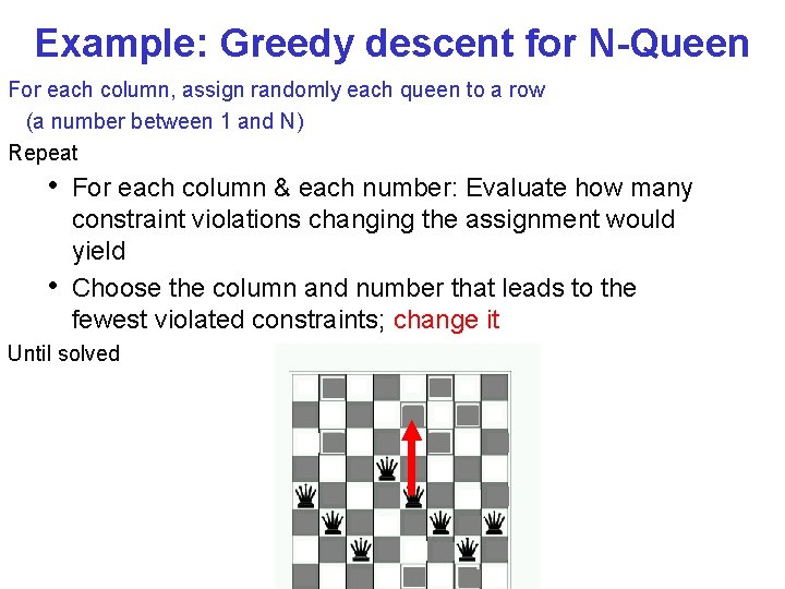
Example: Greedy descent for N-Queen For each column, assign randomly each queen to a row (a number between 1 and N) Repeat • For each column & each number: Evaluate how many • constraint violations changing the assignment would yield Choose the column and number that leads to the fewest violated constraints; change it Until solved

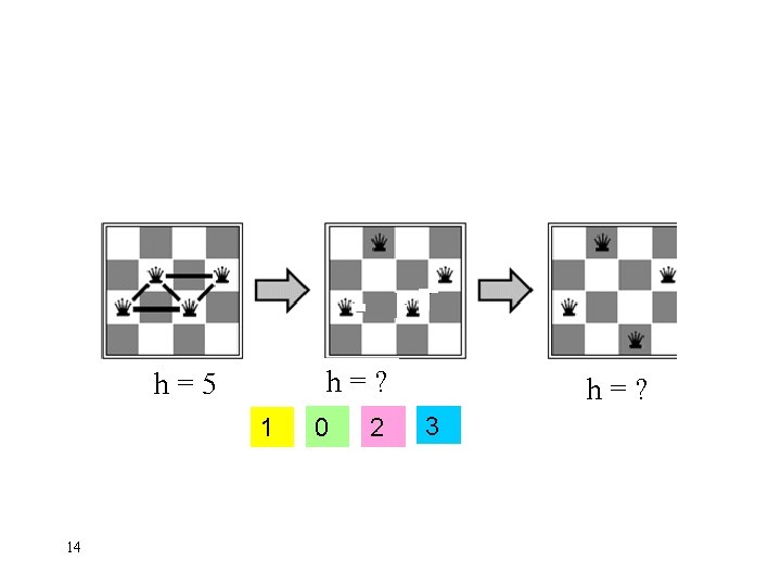
h=? h=5 1 14 0 2 h=? 3

n-queens, Why? Why this problem? Lots of research in the 90’ on local search for CSP was generated by the observation that the run-time of local search on n-queens problems is independent of problem size! CPSC 322, Lecture 5 Slide 15

Lecture Overview • Local search • Constrained Optimization • Greedy Descent / Hill Climbing: Problems • Stochastic Local Search (SLS) • Comparing SLS algorithms • SLS variants üTabu lists üSimulated Annealing • Population Based üBeam search üGenetic Algorithms CPSC 322, Lecture 5 Slide 16

Constrained Optimization Problems So far we have assumed that we just want to find a possible world that satisfies all the constraints. But sometimes solutions may have different values / costs • We want to find the optimal solution that • maximizes the value or • minimizes the cost CPSC 322, Lecture 5 Slide 17

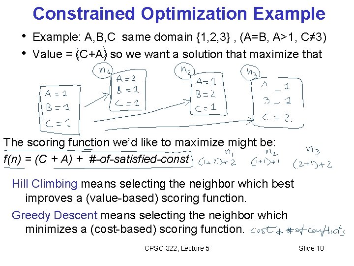
Constrained Optimization Example • Example: A, B, C same domain {1, 2, 3} , (A=B, A>1, C≠ 3) • Value = (C+A) so we want a solution that maximize that The scoring function we’d like to maximize might be: f(n) = (C + A) + #-of-satisfied-const Hill Climbing means selecting the neighbor which best improves a (value-based) scoring function. Greedy Descent means selecting the neighbor which minimizes a (cost-based) scoring function. CPSC 322, Lecture 5 Slide 18

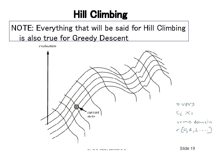
Hill Climbing NOTE: Everything that will be said for Hill Climbing is also true for Greedy Descent CPSC 322, Lecture 5 Slide 19

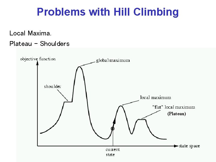
Problems with Hill Climbing Local Maxima. Plateau - Shoulders (Plateau) CPSC 322, Lecture 5 Slide 20

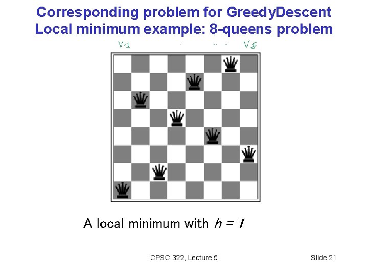
Corresponding problem for Greedy. Descent Local minimum example: 8 -queens problem A local minimum with h = 1 CPSC 322, Lecture 5 Slide 21

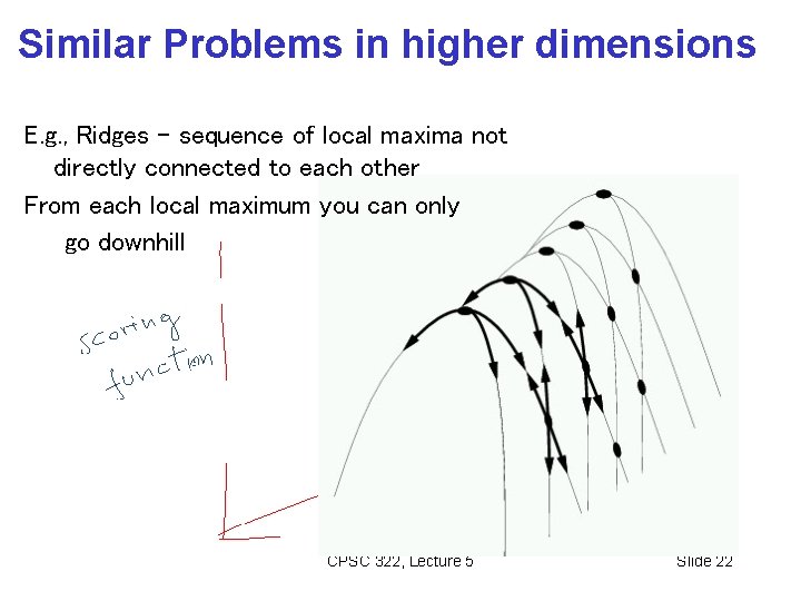
Similar Problems in higher dimensions E. g. , Ridges – sequence of local maxima not directly connected to each other From each local maximum you can only go downhill CPSC 322, Lecture 5 Slide 22

Lecture Overview • Local search • Constrained Optimization • Greedy Descent / Hill Climbing: Problems • Stochastic Local Search (SLS) • Comparing SLS algorithms • SLS variants üTabu lists üSimulated Annealing • Population Based üBeam search üGenetic Algorithms CPSC 322, Lecture 5 Slide 23

Local Search: Summary • A useful method in practice for large CSPs • Start from a possible world • Generate some neighbors ( “similar” possible worlds) • Move from current node to a neighbor, selected to minimize/maximize a scoring function which combines: ü Info about how many constraints are violated/satified ü Information about the cost/quality of the solution (you want the best solution, not just a solution) CPSC 322, Lecture 5 Slide 24

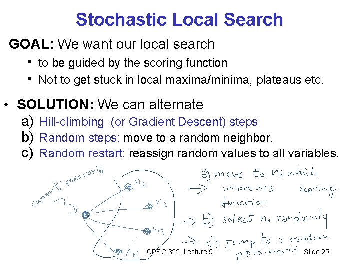
Stochastic Local Search GOAL: We want our local search • to be guided by the scoring function • Not to get stuck in local maxima/minima, plateaus etc. • SOLUTION: We can alternate a) Hill-climbing (or Gradient Descent) steps b) Random steps: move to a random neighbor. c) Random restart: reassign random values to all variables. CPSC 322, Lecture 5 Slide 25

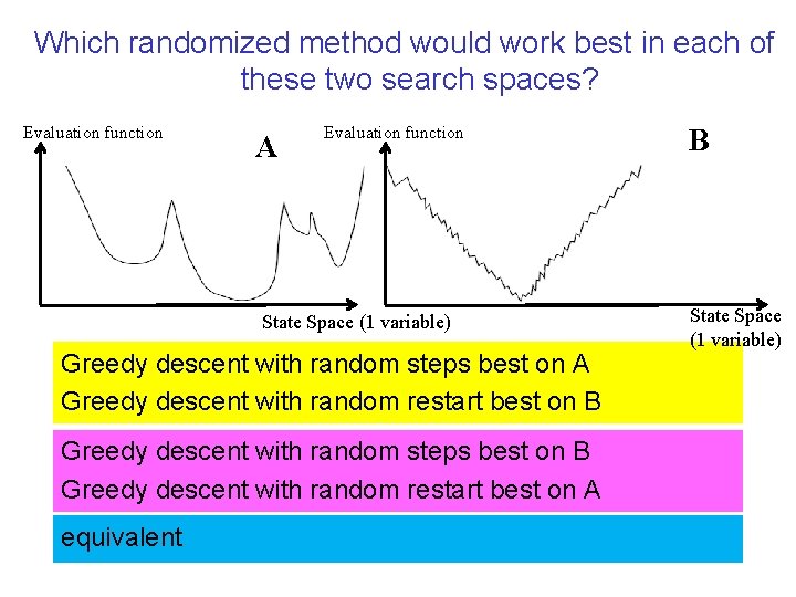
Which randomized method would work best in each of these two search spaces? Evaluation function A Evaluation function State Space (1 variable) Greedy descent with random steps best on A Greedy descent with random restart best on B Greedy descent with random steps best on B Greedy descent with random restart best on A equivalent B State Space (1 variable)

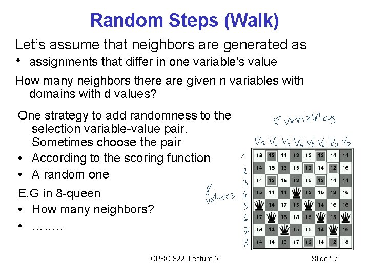
Random Steps (Walk) Let’s assume that neighbors are generated as • assignments that differ in one variable's value How many neighbors there are given n variables with domains with d values? One strategy to add randomness to the selection variable-value pair. Sometimes choose the pair • According to the scoring function • A random one E. G in 8 -queen • How many neighbors? • ……. . CPSC 322, Lecture 5 Slide 27

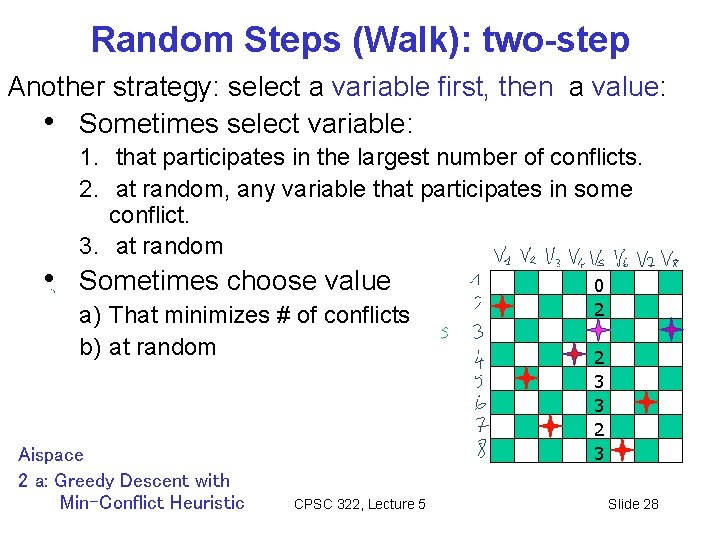
Random Steps (Walk): two-step Another strategy: select a variable first, then a value: • Sometimes select variable: 1. that participates in the largest number of conflicts. 2. at random, any variable that participates in some conflict. 3. at random • Sometimes choose value a) That minimizes # of conflicts b) at random Aispace 2 a: Greedy Descent with Min-Conflict Heuristic CPSC 322, Lecture 5 0 2 2 3 3 2 3 Slide 28

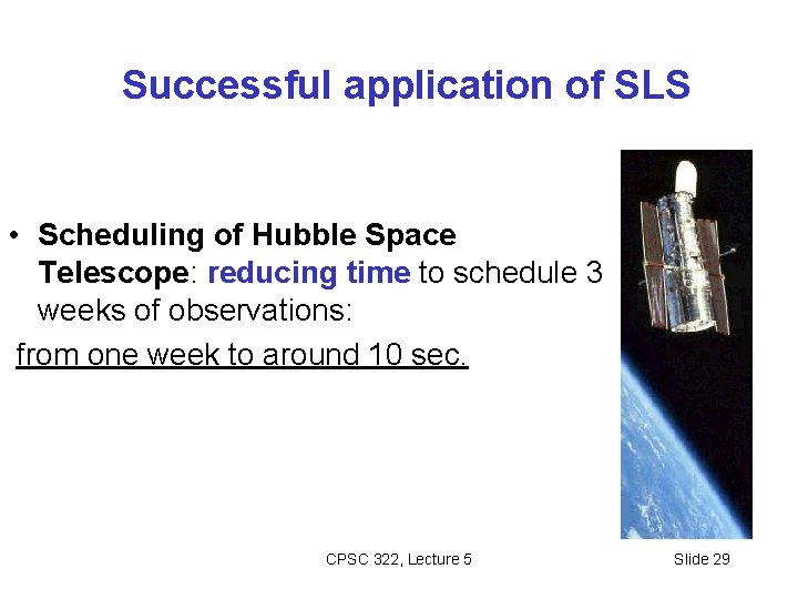
Successful application of SLS • Scheduling of Hubble Space Telescope: reducing time to schedule 3 weeks of observations: from one week to around 10 sec. CPSC 322, Lecture 5 Slide 29

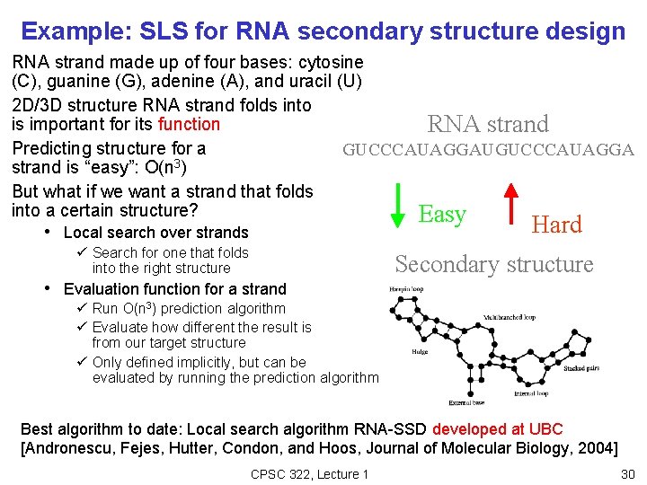
Example: SLS for RNA secondary structure design RNA strand made up of four bases: cytosine (C), guanine (G), adenine (A), and uracil (U) 2 D/3 D structure RNA strand folds into is important for its function RNA strand Predicting structure for a GUCCCAUAGGAUGUCCCAUAGGA 3 strand is “easy”: O(n ) But what if we want a strand that folds into a certain structure? Easy Hard • Local search over strands ü Search for one that folds into the right structure • Evaluation function for a strand Secondary structure ü Run O(n 3) prediction algorithm ü Evaluate how different the result is from our target structure ü Only defined implicitly, but can be evaluated by running the prediction algorithm Best algorithm to date: Local search algorithm RNA-SSD developed at UBC [Andronescu, Fejes, Hutter, Condon, and Hoos, Journal of Molecular Biology, 2004] CPSC 322, Lecture 1 30

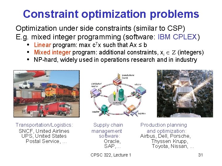
Constraint optimization problems Optimization under side constraints (similar to CSP) E. g. mixed integer programming (software: IBM CPLEX) • Linear program: max c. Tx such that Ax ≤ b • Mixed integer program: additional constraints, xi Z (integers) • NP-hard, widely used in operations research and in industry Transportation/Logistics: SNCF, United Airlines UPS, United States Postal Service, … Supply chain management software: Oracle, SAP, … CPSC 322, Lecture 1 Production planning and optimization: Airbus, Dell, Porsche, Thyssen Krupp, Toyota, Nissan, . . . 31

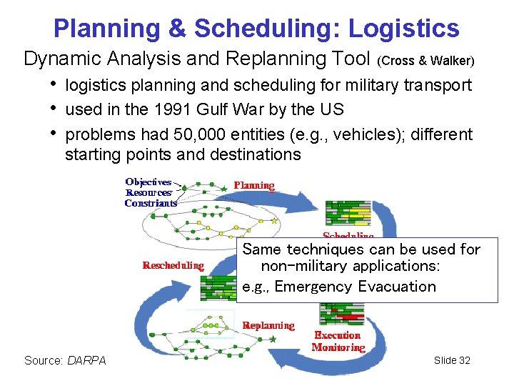
Planning & Scheduling: Logistics Dynamic Analysis and Replanning Tool (Cross & Walker) • logistics planning and scheduling for military transport • used in the 1991 Gulf War by the US • problems had 50, 000 entities (e. g. , vehicles); different starting points and destinations Same techniques can be used for non-military applications: e. g. , Emergency Evacuation Source: DARPA CPSC 322, Lecture 1 Slide 32

CSP/logic: formal verification Hardware verification (e. g. , IBM) Software verification (small to medium programs) Most progress in the last 10 years based on: Encodings into propositional satisfiability (SAT) CPSC 322, Lecture 1 33

(Stochastic) Local search advantage: Online setting • When the problem can change (particularly important in scheduling) • E. g. , schedule for airline: thousands of flights and thousands of personnel assignment • Storm can render the schedule infeasible • Goal: Repair with minimum number of changes • This can be easily done with a local search starting form the current schedule • Other techniques usually: • require more time • might find solution requiring many 5 more changes CPSC 322, Lecture Slide 34

SLS limitations • Typically no guarantee to find a solution even if one exists • SLS algorithms can sometimes stagnate üGet caught in one region of the search space and never terminate • Very hard to analyze theoretically • Not able to show that no solution exists • SLS simply won’t terminate • You don’t know whether the problem is infeasible or the algorithm has stagnated

SLS Advantage: anytime algorithms • When should the algorithm be stopped ? • When a solution is found • • (e. g. no constraint violations) Or when we are out of time: you have to act NOW Anytime algorithm: ümaintain the node with best h found so far (the “incumbent”) ügiven more time, can improve its incumbent

Learning Goals for today’s class – part 1 You can: • Implement local search for a CSP. • Implement different ways to generate neighbors • Implement scoring functions to solve a CSP by local search through either greedy descent or hill-climbing. • Implement SLS with • random steps (1 -step, 2 -step versions) • random restart CPSC 322, Lecture 5 Slide 37

Lecture Overview • Local search • Constrained Optimization • Greedy Descent / Hill Climbing: Problems • Stochastic Local Search (SLS) • Comparing SLS algorithms • SLS variants üTabu lists üSimulated Annealing • Population Based üBeam search üGenetic Algorithms CPSC 322, Lecture 5 Slide 38

Evaluating SLS algorithms • SLS algorithms are randomized • The time taken until they solve a problem is a random variable • It is entirely normal to have runtime variations of 2 orders of magnitude in repeated runs! ü E. g. 0. 1 seconds in one run, 10 seconds in the next one ü On the same problem instance (only difference: random seed) ü Sometimes SLS algorithm doesn’t even terminate at all: stagnation • If an SLS algorithm sometimes stagnates, what is its mean runtime (across many runs)? • Infinity! • In practice, one often counts timeouts as some fixed large value X • Still, summary statistics, such as mean run time or median run time, don't tell the whole story ü E. g. would penalize an algorithm that often finds a solution quickly but sometime stagnates

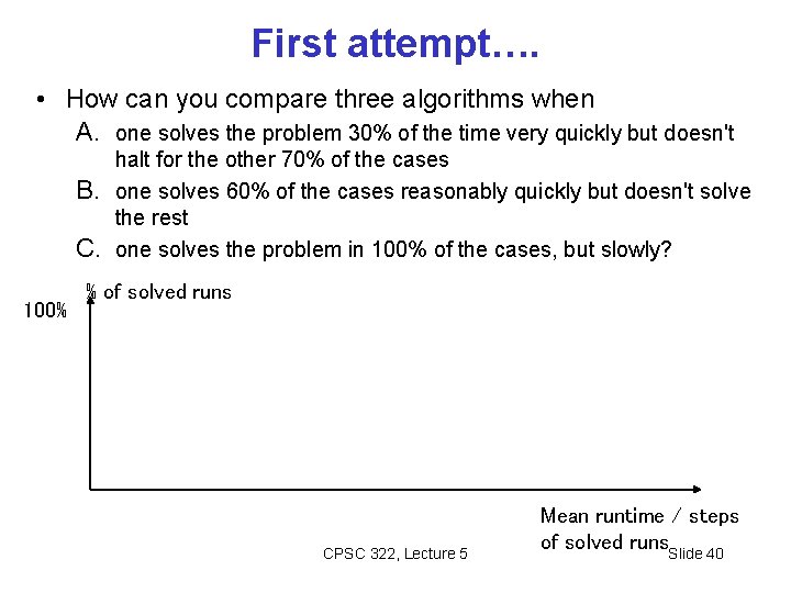
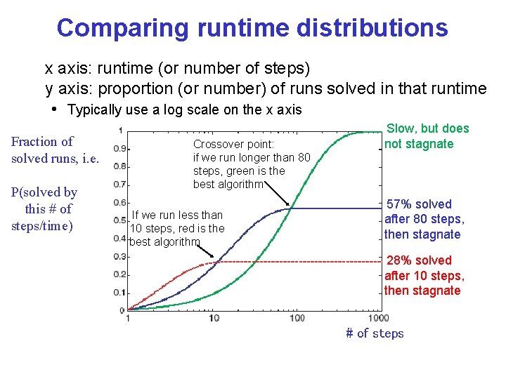
First attempt…. • How can you compare three algorithms when A. one solves the problem 30% of the time very quickly but doesn't B. C. 100% halt for the other 70% of the cases one solves 60% of the cases reasonably quickly but doesn't solve the rest one solves the problem in 100% of the cases, but slowly? % of solved runs CPSC 322, Lecture 5 Mean runtime / steps of solved runs. Slide 40

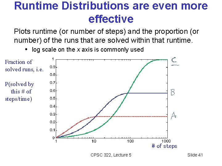
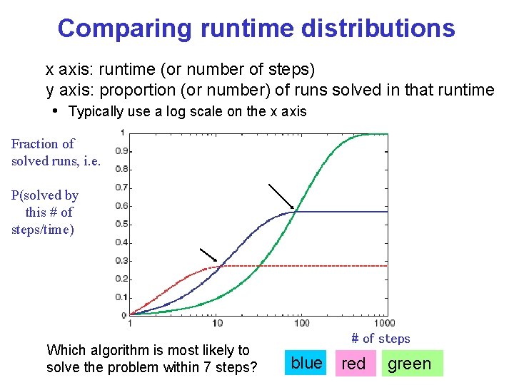
Runtime Distributions are even more effective Plots runtime (or number of steps) and the proportion (or number) of the runs that are solved within that runtime. • log scale on the x axis is commonly used Fraction of solved runs, i. e. P(solved by this # of steps/time) # of steps CPSC 322, Lecture 5 Slide 41

Comparing runtime distributions x axis: runtime (or number of steps) y axis: proportion (or number) of runs solved in that runtime • Typically use a log scale on the x axis Fraction of solved runs, i. e. P(solved by this # of steps/time) Which algorithm is most likely to solve the problem within 7 steps? # of steps blue red green

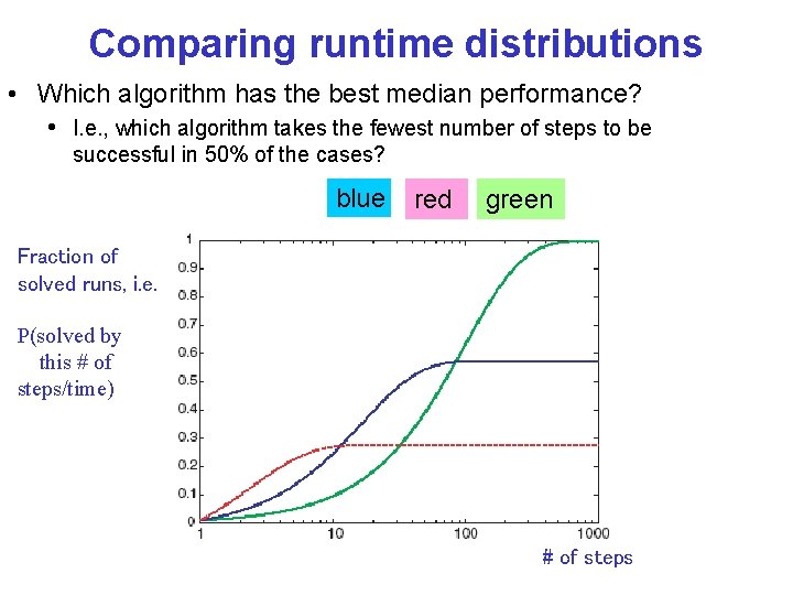
Comparing runtime distributions • Which algorithm has the best median performance? • I. e. , which algorithm takes the fewest number of steps to be successful in 50% of the cases? blue red green Fraction of solved runs, i. e. P(solved by this # of steps/time) # of steps

Comparing runtime distributions x axis: runtime (or number of steps) y axis: proportion (or number) of runs solved in that runtime • Typically use a log scale on the x axis Fraction of solved runs, i. e. P(solved by this # of steps/time) Crossover point: if we run longer than 80 steps, green is the best algorithm If we run less than 10 steps, red is the best algorithm Slow, but does not stagnate 57% solved after 80 steps, then stagnate 28% solved after 10 steps, then stagnate # of steps

Runtime distributions in AIspace • Let’s look at some algorithms and their runtime distributions: 1. Greedy Descent 2. Random Sampling 3. Random Walk 4. Greedy Descent with random walk • Simple scheduling problem 2 in AIspace:

Stochastic Local Search • Key Idea: combine greedily improving moves with randomization • As well as improving steps we can allow a “small probability” of: • Random steps: move to a random neighbor. • Random restart: reassign random values to all variables. • Always keep best solution found so far • Stop when • Solution is found (in vanilla CSP ……………) • Run out of time (return best solution so far) CPSC 322, Lecture 5 Slide 48

Lecture Overview • Local search • Constrained Optimization • Greedy Descent / Hill Climbing: Problems • Stochastic Local Search (SLS) • Comparing SLS algorithms • SLS variants üTabu lists üSimulated Annealing • Population Based üBeam search üGenetic Algorithms CPSC 322, Lecture 5 Slide 49

Tabu lists • To avoid search to • Immediately going back to previously visited candidate • To prevent cycling • Maintain a tabu list of the k last nodes visited. • Don't visit a poss. world that is already on the tabu list. • Cost of this method depends on…. . CPSC 322, Lecture 5 Slide 50

Simulated Annealing • Key idea: Change the degree of randomness…. • Annealing: a metallurgical process where metals are hardened by being slowly cooled. • Analogy: start with a high ``temperature'': a high tendency to take random steps • Over time, cool down: more likely to follow the scoring function • Temperature reduces over time, according to an annealing schedule CPSC 322, Lecture 5 Slide 51

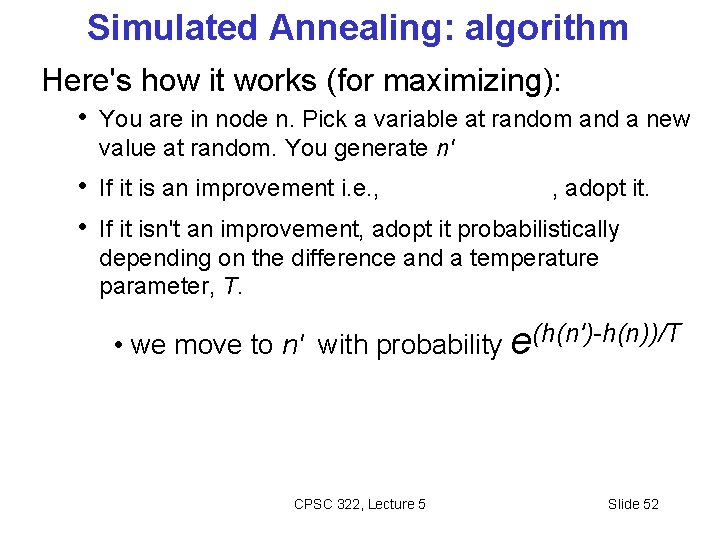
Simulated Annealing: algorithm Here's how it works (for maximizing): • You are in node n. Pick a variable at random and a new value at random. You generate n' • If it is an improvement i. e. , , adopt it. • If it isn't an improvement, adopt it probabilistically depending on the difference and a temperature parameter, T. • we move to n' with probability e(h(n')-h(n))/T CPSC 322, Lecture 5 Slide 52

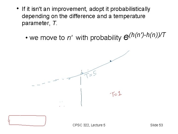
• If it isn't an improvement, adopt it probabilistically depending on the difference and a temperature parameter, T. • we move to n' with probability e(h(n')-h(n))/T CPSC 322, Lecture 5 Slide 53

Properties of simulated annealing search One can prove: If T decreases slowly enough, then simulated annealing search will find a global optimum with probability approaching 1 Widely used in VLSI layout, airline scheduling, etc. CPSC 322, Lecture 5 Slide 54

Lecture Overview • Local search • Constrained Optimization • Greedy Descent / Hill Climbing: Problems • Stochastic Local Search (SLS) • Comparing SLS algorithms • SLS variants üTabu lists üSimulated Annealing • Population Based üBeam search üGenetic Algorithms CPSC 322, Lecture 5 Slide 55

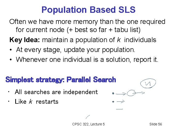
Population Based SLS Often we have more memory than the one required for current node (+ best so far + tabu list) Key Idea: maintain a population of k individuals • At every stage, update your population. • Whenever one individual is a solution, report it. Simplest strategy: Parallel Search • All searches are independent • Like k restarts CPSC 322, Lecture 5 Slide 56

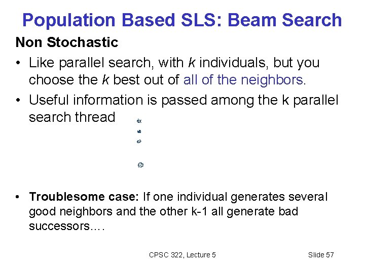
Population Based SLS: Beam Search Non Stochastic • Like parallel search, with k individuals, but you choose the k best out of all of the neighbors. • Useful information is passed among the k parallel search thread • Troublesome case: If one individual generates several good neighbors and the other k-1 all generate bad successors…. CPSC 322, Lecture 5 Slide 57

Population Based SLS: Stochastic Beam Search • Non Stochastic Beam Search may suffer from lack of diversity among the k individual (just a more expensive hill climbing) • Stochastic version alleviates this problem: • Selects the k individuals at random • But probability of selection proportional to their value (according to scoring function) CPSC 322, Lecture 5 Slide 58

Stochastic Beam Search: Advantages • It maintains diversity in the population. • Biological metaphor (asexual reproduction): üeach individual generates “mutated” copies of itself (its neighbors) üThe scoring function value reflects the fitness of the individual üthe higher the fitness the more likely the individual will survive (i. e. , the neighbor will be in the next generation) CPSC 322, Lecture 5 Slide 59

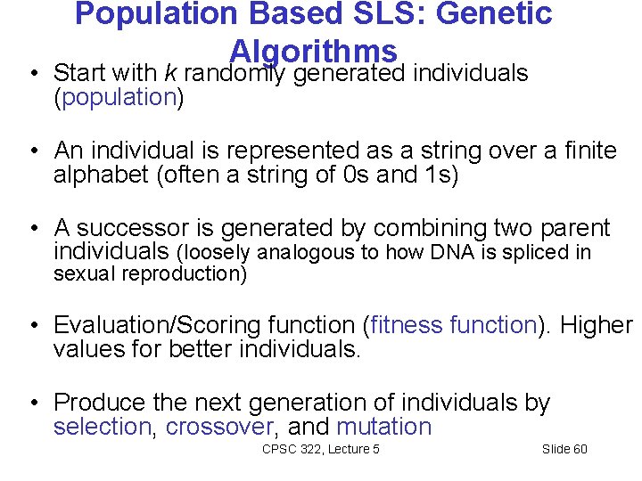
Population Based SLS: Genetic Algorithms • Start with k randomly generated individuals (population) • An individual is represented as a string over a finite alphabet (often a string of 0 s and 1 s) • A successor is generated by combining two parent individuals (loosely analogous to how DNA is spliced in sexual reproduction) • Evaluation/Scoring function (fitness function). Higher values for better individuals. • Produce the next generation of individuals by selection, crossover, and mutation CPSC 322, Lecture 5 Slide 60

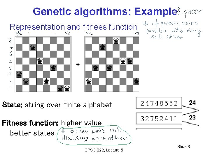
Genetic algorithms: Example Representation and fitness function State: string over finite alphabet Fitness function: higher value better states CPSC 322, Lecture 5 Slide 61

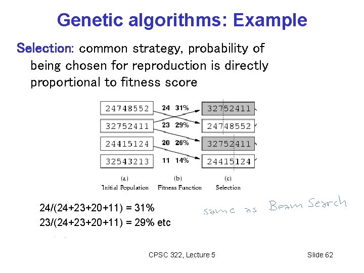
Genetic algorithms: Example Selection: common strategy, probability of being chosen for reproduction is directly proportional to fitness score 24/(24+23+20+11) = 31% 23/(24+23+20+11) = 29% etc CPSC 322, Lecture 5 Slide 62

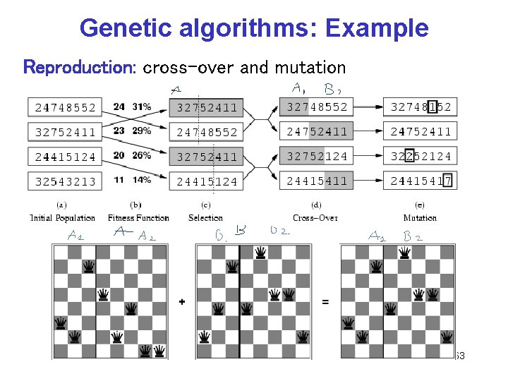
Genetic algorithms: Example Reproduction: cross-over and mutation CPSC 322, Lecture 5 Slide 63

Genetic Algorithms: Conclusions • Their performance is very sensitive to the choice of state representation and fitness function • Extremely slow (not surprising as they are inspired by evolution!) CPSC 322, Lecture 5 Slide 64

Learning Goals for today’s class part 2 You can: • Compare SLS algorithms with runtime distributions • Implement a tabu-list. • Implement the simulated annealing algorithm • Implement population based SLS algorithms: • Beam Search • Genetic Algorithms. • Explain pros and cons of different SLS algorithms. CPSC 322, Lecture 5 Slide 65

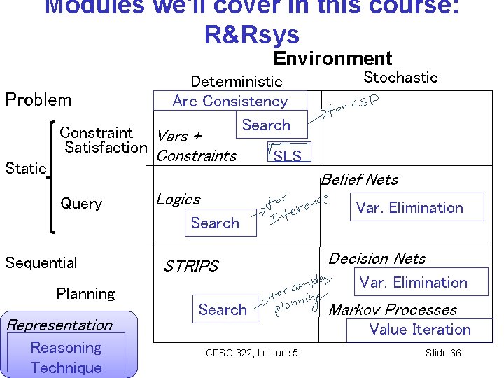
Modules we'll cover in this course: R&Rsys Environment Problem Static Deterministic Arc Consistency Search Constraint Vars + Satisfaction Constraints Stochastic SLS Belief Nets Query Logics Search Sequential Planning Representation Reasoning Technique STRIPS Search Var. Elimination Decision Nets Var. Elimination Markov Processes Value Iteration CPSC 322, Lecture 5 Slide 66

Next class Posted on Web. CT • Assignment 2 on CSPs (due on Thurs!) • Planning (Chp 8. 1 -8. 2, 8. 4): How to select and organize a sequence of actions to achieve a given goal… • Start Logics (Chp 5 -1 -5. 3) CPSC 322, Lecture 5 Slide 67

Sampling a discrete probability distribution CPSC 322, Lecture 5 Slide 68

Systematically solving CSPs: Summary • Build Constraint Network • Apply Arc Consistency • One domain is empty • Each domain has a single value • Some domains have more than one value • Apply Depth-First Search with Pruning • Split the problem in a number of disjoint cases • Apply Arc Consistency to each case CPSC 322, Lecture 5 Slide 69

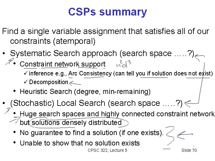
CSPs summary Find a single variable assignment that satisfies all of our constraints (atemporal) • Systematic Search approach (search space …. . ? ) • Constraint network support ü inference e. g. , Arc Consistency (can tell you if solution does not exist) ü Decomposition • Heuristic Search (degree, min-remaining) • (Stochastic) Local Search (search space …. . ? ) • Huge search spaces and highly connected constraint network • • but solutions densely distributed No guarantee to find a solution (if one exists). Unable to show that no solution exists CPSC 322, Lecture 5 Slide 70

Local Search: Motivation • Solving CSPs is NP-hard - Search space for many CSPs is huge - Exponential in the number of variables - Even arc consistency with domain splitting is often not enough • Alternative: local search • use algorithms that search the space locally, rather than systematically • Often finds a solution quickly, but are not guaranteed to find a solution if one exists (thus, cannot prove that there is no solution)

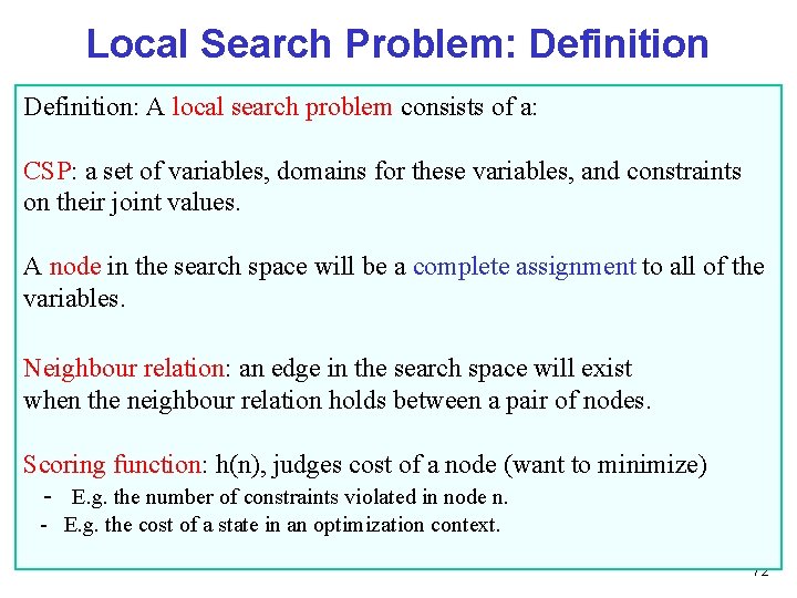
Local Search Problem: Definition: A local search problem consists of a: CSP: a set of variables, domains for these variables, and constraints on their joint values. A node in the search space will be a complete assignment to all of the variables. Neighbour relation: an edge in the search space will exist when the neighbour relation holds between a pair of nodes. Scoring function: h(n), judges cost of a node (want to minimize) - E. g. the number of constraints violated in node n. - E. g. the cost of a state in an optimization context. 72

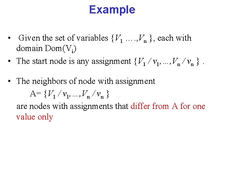
Example • Given the set of variables {V 1 …. , Vn }, each with domain Dom(Vi) • The start node is any assignment {V 1 / v 1, …, Vn / vn }. • The neighbors of node with assignment A= {V 1 / v 1, …, Vn / vn } are nodes with assignments that differ from A for one value only

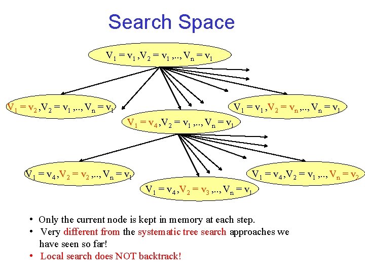
Search Space V 1 = v 1 , V 2 = v 1 , . . , Vn = v 1 V 1 = v 2 , V 2 = v 1 , . . , Vn = v 1 V 1 = v 1 , V 2 = vn , . . , Vn = v 1 V 1 = v 4 , V 2 = v 1 , . . , Vn = v 1 V 1 = v 4 , V 2 = v 2 , . . , Vn = v 1 V 1 = v 4 , V 2 = v 1 , . . , Vn = v 2 V 1 = v 4 , V 2 = v 3 , . . , Vn = v 1 • Only the current node is kept in memory at each step. • Very different from the systematic tree search approaches we have seen so far! • Local search does NOT backtrack!